# Instructor dataset guide
## Generating truth, models, and analysis results
63 methods · simulated data · saved analysis results
All records are simulated. Generating truth is stated from the model, independently of the sample p-value. A true effect can yield a large p-value; a true null can yield a small one.
CSV rows are not automatically the independent sample size. Use each dataset's design to identify pairing, repeated observations, clustering, or aggregation.
[Dataset catalog](dataset_catalog.csv)
## Quick index
| Method | Biological scenario | Rows | Seed | Generating truth | Saved result | CSV |
|---|---|---:|---:|---|---|---|
| [One-sample t test](#dataset-one_sample_t) | Cell biologists measure oxygen consumption in independently cultured cell lines. | 24 | 1101 | The population mean is 10.8 nmol/min, so the reference-mean null of 10 is false; the true mean difference is +0.8. | Mean = 10.75 nmol/min; n = 24 t = 2.48; df = 23; p = 0.02107 | [CSV](modules/one_sample_t/generated/data.csv) |
| [Pooled two-sample t test](#dataset-pooled_t) | Evolutionary biologists compare adult beetle body length from two rearing environments. | 56 | 1118 | The true Cool minus Warm mean difference is -0.7 mm, and the two population variances are both 0.4225 mm squared. | Cool - Warm mean difference = -1.02 mm Pooled t = -4.94; df = 54.00; p = 7.927e-06 | [CSV](modules/pooled_t/generated/data.csv) |
| [Welch two-sample t test](#dataset-welch_t) | Evolutionary biologists compare adult beetle body length from two rearing environments. | 56 | 1102 | The true Cool minus Warm mean difference is -0.7 mm. Variances differ (0.4225 versus 1.3225 mm squared). | Cool - Warm mean difference = -1.01 mm Welch t = -4.21; df = 53.33; p = 9.973e-05 | [CSV](modules/welch_t/generated/data.csv) |
| [Paired t test](#dataset-paired_t) | Plant physiologists measure photosynthesis in the same leaves before and after heat stress. | 20 | 1103 | The mean after-minus-before difference is -1.3 photosynthesis units, even if this sample provides limited evidence against zero. | Mean change (after - before) = -0.73 Paired t = -1.91; df = 19; p = 0.07128 | [CSV](modules/paired_t/generated/data.csv) |
| [F test of two variances](#dataset-f_variance) | Evolutionary developmental biologists compare variation in wing length between two inbred fly lines. | 60 | 1109 | Population means are equal, but the true variance ratio A/B is 0.11 squared / 0.21 squared, approximately 0.274. | Variance ratio (A / B) = 0.376 F = 0.376; df = 29, 29; p = 0.01048 | [CSV](modules/f_variance/generated/data.csv) |
| [Levene and Brown–Forsythe tests](#dataset-levene) | Microbiologists compare the variability of colony diameters across three nutrient media. | 84 | 1110 | Group geometric means are 4 mm, but variances differ. Arithmetic means also vary slightly because log-normal means depend on log-scale spread. | Brown–Forsythe F = 5.55; df = 2, 81; p = 0.005524 Original Levene F = 9.72; p = 0.0001645 | [CSV](modules/levene/generated/data.csv) |
| [Shapiro–Wilk and graphical checks](#dataset-shapiro) | Cell biologists examine the distribution of time to lysis among independent cultured cells. | 36 | 1111 | The population is log-normal and positively skewed, not normal. The population geometric mean is 45 minutes. | Shapiro–Wilk W = 0.937; p = 0.04064; n = 36 Curvature in the Q–Q plot indicates a shape mismatch. | [CSV](modules/shapiro/generated/data.csv) |
| [Sign test](#dataset-sign_test) | Behavioral biologists record the change in refuge-use time after a predator cue. | 30 | 1104 | Positive changes are more likely than negative changes. The unrounded mean is 4 seconds, but the sign test is about direction rather than that mean. | Positive changes: 18 of 30 nonzero differences Exact two-sided p = 0.3616 | [CSV](modules/sign_test/generated/data.csv) |
| [Wilcoxon signed-rank test](#dataset-signed_rank) | Microbiologists compare log bacterial density before and after a treatment in matched cultures. | 28 | 1105 | The symmetric difference distribution is centered at +0.28 log10 units; its zero-center null is false. | Pseudomedian change estimate = 0.249 V = 328.0; p = 0.004582 | [CSV](modules/signed_rank/generated/data.csv) |
| [Wilcoxon rank-sum test](#dataset-rank_sum) | Ecologists compare parasite burdens among fish from two independent lakes. | 64 | 1106 | The lake distributions differ, including their mean and spread. The same-distribution null is false; there is not a simple equal-shape location shift. | Observed medians: Clear 3.0; Reedy 8.0 parasites W = 362.5; asymptotic p = 0.04452 | [CSV](modules/rank_sum/generated/data.csv) |
| [One-way ANOVA](#dataset-one_way_anova) | Ecologists compare seedling biomass under three independent soil treatments. | 75 | 1117 | The equal-means null is false. All three populations share variance 0.85 squared; Loam minus Sand is truly 0.9 g. | Ordinary ANOVA F(2, 72) = 11.59; p = 4.335e-05 Welch ANOVA F = 8.89; denominator df = 46.37; p = 0.0005408 | [CSV](modules/one_way_anova/generated/data.csv) |
| [Welch one-way ANOVA](#dataset-welch_anova) | Ecologists compare seedling biomass under three independent soil treatments. | 78 | 1119 | The true means differ, and variances differ (0.36, 1.21, and 2.25 g squared). Welch addresses the equal-means null without a shared variance. | Welch ANOVA F = 13.65; df = 2, 49.85; p = 1.873e-05 Group sample sizes: Sand 20; Loam 26; Clay 32 | [CSV](modules/welch_anova/generated/data.csv) |
| [Kruskal–Wallis test](#dataset-kruskal_wallis) | Plant pathologists score leaf damage in three independently assigned pathogen treatments. | 72 | 1107 | The score distributions differ across all three generating probabilities; expected scores are 2.0, 3.2, and 4.64. The equal-distributions null is false. | Kruskal–Wallis chi-square = 35.75; df = 2; p = 1.73e-08 Observed medians: Control 2; Strain A 3; Strain B 4.5 | [CSV](modules/kruskal_wallis/generated/data.csv) |
| [Factorial ANOVA: interactions](#dataset-factorial_anova) | Beetle larvae from two genotypes are independently reared at two temperatures. | 88 | 2101 | The temperature effect is 2 mg/week in genotype A and 4.3 mg/week in B, so the interaction is 2.3 mg/week. The interaction null is false. | Interaction = 4.30 mg/week t(84) = 5.69; p = 1.78e-07 | [CSV](modules/factorial_anova/generated/data.csv) |
| [ANCOVA: an adjusted group comparison](#dataset-ancova) | Plant ecologists compare nutrient treatment while accounting for initial plant height. | 90 | 2102 | The nutrient treatment increases the population mean biomass by 2.4 g at any shared initial height. Both groups have slope 1.5 g/cm. The adjusted treatment null is false. | Adjusted nutrient minus control = 2.65 g t(87) = 6.55; p = 3.797e-09 | [CSV](modules/ancova/generated/data.csv) |
| [Repeated-measures ANOVA](#dataset-repeated_anova) | Physiologists measure the same animals at four assay temperatures. | 96 | 2103 | Population means are 8, 9.75, 11.5 and 13.25 µmol/hour. The endpoint difference is 5.25 µmol/hour and the equal-means null is false. | Condition F(3, 69) = 84.32 Omnibus p = 4.966e-23 | [CSV](modules/repeated_anova/generated/data.csv) |
| [Friedman test](#dataset-friedman) | Sensory biologists record activity scores from each insect under three light conditions. | 54 | 1108 | Condition effects exist before rounding (0, +0.8, +1.6), and condition score distributions differ after rounding. Repeated observations share an insect baseline. | Independent blocks = 18; conditions = 3 Friedman chi-square = 17.63; df = 2; p = 0.0001482 | [CSV](modules/friedman/generated/data.csv) |
| [Tukey / Tukey–Kramer comparisons](#dataset-tukey) | Plant growth is compared across four nutrient regimes. | 80 | 2104 | Population means for A–D are 8, 9, 11.3 and 12.1 g; all distinct pairwise mean-equality nulls are false. | Family: all six pairwise nutrient comparisons Tukey-adjusted p = 0.0415 | [CSV](modules/tukey/generated/data.csv) |
| [Fisher least significant difference](#dataset-fisher_lsd) | Plant growth is compared across four nutrient regimes. | 80 | 2104 | Population means for A–D are 8, 9, 11.3 and 12.1 g; all distinct pairwise mean-equality nulls are false. | Omnibus p = 5.683e-12 Unadjusted p = 0.05163 | [CSV](modules/fisher_lsd/generated/data.csv) |
| [Scheffé contrasts](#dataset-scheffe) | Plant growth is compared across four nutrient regimes. | 80 | 2104 | Population means for A–D are 8, 9, 11.3 and 12.1 g; all distinct pairwise mean-equality nulls are false. The specified (C+D)/2 − (A+B)/2 contrast equals 3.2 g. | Contrast: (C + D)/2 − (A + B)/2 Scheffé-adjusted p = 9.177e-11 | [CSV](modules/scheffe/generated/data.csv) |
| [Dunn rank comparisons](#dataset-dunn) | Ecologists compare skewed leaf-damage measurements among four treatments. | 84 | 2105 | Group distributions differ; their population medians are exp(1.2), exp(1.3), exp(1.7) and exp(1.9) mm². Dunn tests pooled-rank tendencies, not arithmetic mean equality. The distributions also differ in original-scale spread. | Kruskal–Wallis p = 1.352e-05 Two-sided Holm-adjusted p = 0.0001018 | [CSV](modules/dunn/generated/data.csv) |
| [Pearson correlation](#dataset-pearson) | Evolutionary biologists measure wing and tail lengths in adult birds from a single population. | 45 | 1112 | The generating population Pearson correlation is 0.55*5 / sqrt((0.55*5)^2 + 3.5^2), approximately 0.618. It is not the observed sample correlation. | Pearson r = 0.700 t = 6.43; df = 43; p = 8.606e-08 | [CSV](modules/pearson/generated/data.csv) |
| [Spearman rank correlation](#dataset-spearman) | Microbial ecologists compare soil salinity with bacterial richness across independent soil cores. | 45 | 1113 | The underlying mean response decreases nonlinearly with salinity, creating a negative monotonic association. No fixed numeric population Spearman coefficient was specified. | Spearman rho = -0.752; n = 45 S = 26599.8; asymptotic two-sided p = 2.549e-09 | [CSV](modules/spearman/generated/data.csv) |
| [Simple linear regression](#dataset-simple_lm) | Plant ecologists grow seedlings under a gradient of nitrogen supply. | 36 | 1114 | The conditional mean intercept is 2.2 g and slope is +0.42 g per mg nitrogen. The zero-slope null is false. | Slope = 0.414 g biomass per mg nitrogen Slope t = 9.90; df = 34; p = 1.525e-11 | [CSV](modules/simple_lm/generated/data.csv) |
| [Multiple linear regression](#dataset-multiple_lm) | Evolutionary biologists relate beetle horn length to body size and larval nutrition. | 60 | 1115 | The true conditional body slope is 0.35 mm/mm and nutrition slope 0.16 mm/mg, with no interaction. Both zero-coefficient nulls are false. | Body slope, adjusted for nutrition = 0.299 mm/mm Body coefficient p = 7.658e-05; nested-model F = 18.17 | [CSV](modules/multiple_lm/generated/data.csv) |
| [Theil–Sen robust slope](#dataset-theil_sen) | Physiologists measure enzyme activity along a temperature gradient with occasional unusually high assays. | 40 | 1116 | The underlying uncontaminated linear trend has slope 1.4 U/mL per degree C. Two deliberately elevated assays illustrate robustness; the bootstrap interval comes from the saved contaminated sample. | Theil–Sen slope = 1.408 U/mL per degree C 95% pairs-bootstrap interval: 1.184 to 1.618 | [CSV](modules/theil_sen/generated/data.csv) |
| [Exact binomial test](#dataset-binomial) | Host choice in a parasitoid wasp | 80 | 3101 | The true native-host probability is 0.68, so the null probability 0.50 is false. The population difference from the null is +0.18. | Native-host choices: 51 / 80 Exact two-sided p = 0.01832 | [CSV](modules/binomial/generated/data.csv) |
| [One-proportion test](#dataset-one_proportion) | Germination of salt-tolerant seeds | 120 | 3102 | The true germination probability is 0.67 rather than the null benchmark 0.50; the population difference is +0.17. | Germination: 70 / 120 Two-sided p = 0.06789 | [CSV](modules/one_proportion/generated/data.csv) |
| [Two-proportion test](#dataset-two_proportions) | Heat survival in evolved and ancestral yeast | 220 | 3103 | Evolved minus ancestral survival probability is 0.20, so the equal-probabilities null is false. The corresponding population odds ratio is approximately 2.37. | Evolved: 78 / 110; ancestral: 61 / 110 Two-sided p = 0.01748 | [CSV](modules/two_proportions/generated/data.csv) |
| [Chi-square goodness-of-fit](#dataset-chi_gof) | Segregation in an F2 cross | 240 | 3104 | The simulated probabilities differ from 1:2:1 by -0.07, +0.04, and +0.03. The goodness-of-fit null is false. | Observed: 43, 128, 69 p = 0.03508 | [CSV](modules/chi_gof/generated/data.csv) |
| [Chi-square test of independence](#dataset-chi_independence) | Infection across three lizard habitats | 270 | 3105 | Infection probability depends on habitat, so the independence null is false. Urban minus forest infection probability is 0.30; the simulation does not assign causality to habitat. | Infection probabilities: Forest 0.14; Grassland 0.41; Urban 0.54 p = 1.042e-07; Cramer V = 0.345 | [CSV](modules/chi_independence/generated/data.csv) |
| [Fisher exact test](#dataset-fisher_exact) | Survival of rare resistant and susceptible clones | 24 | 3106 | The resistant-to-susceptible population survival odds ratio is (0.65/0.35)/(0.20/0.80), approximately 7.43. The odds-ratio-one null is false. | Survivors: susceptible 2/12; resistant 7/12 Two-sided exact p = 0.08938 | [CSV](modules/fisher_exact/generated/data.csv) |
| [McNemar test](#dataset-mcnemar) | Antibody detection before and after an exposure season | 80 | 3107 | Marginal after positivity is 0.45×0.85 + 0.55×0.35 = 0.575, a +0.125 change from before. Population gain and loss probabilities are 0.1925 and 0.0675, so the McNemar null is false. | Gained detection: 10; lost detection: 5 McNemar p = 0.1967; exact paired p = 0.3018 | [CSV](modules/mcnemar/generated/data.csv) |
| [Cochran’s Q test](#dataset-cochran_q) | Bee visits to three floral odors | 180 | 3108 | Increasing odor effects produce strictly increasing marginal visit probabilities across A, B, and C. The equal-probabilities null is false; the latent log-odds differences are not themselves the marginal probability differences. | Matched bees: 60; conditions: 3 Omnibus p = 0.07643 | [CSV](modules/cochran_q/generated/data.csv) |
| [Logistic regression](#dataset-logistic) | Hybrid viability across parental divergence | 160 | 3110 | The true divergence coefficient is -0.5; viability odds are multiplied by exp(-0.5) ≈ 0.607 per divergence percentage point. The zero-slope null is false. The probability decline is nonlinear. | Divergence coefficient: -0.464 Likelihood-ratio p = 6.573e-09 | [CSV](modules/logistic/generated/data.csv) |
| [Exact Poisson rate test](#dataset-poisson_exact) | De novo mutations in sequenced microbial lineages | 60 | 3109 | The true rate is 0.40 mutations/Mb rather than the null rate 0.25/Mb. The population rate ratio to the null is 1.6. | Events: 345; exposure: 845.0 Mb Exact p = 3.246e-17 | [CSV](modules/poisson_exact/generated/data.csv) |
| [Poisson regression](#dataset-poisson_glm) | Coral recruit counts and live coral cover | 120 | 3111 | The true cover coefficient is 0.016. A 10-point cover increase multiplies recruit density by exp(0.16) ≈ 1.174. The zero-slope null is false, and the exposure coefficient is fixed at one. | Rate ratio per 10 cover points: 1.200 Likelihood-ratio p = 2.64e-30 | [CSV](modules/poisson_glm/generated/data.csv) |
| [Quasi-Poisson regression](#dataset-quasipoisson) | Bacterial colony counts with clumping | 120 | 3113 | High medium multiplies mean colony density by exp(0.5) ≈ 1.649; the equal-rate null is false. The true dispersion multiplier is 4, so Poisson uncertainty would be too small. | High / low mean rate ratio: 1.351 Quasi-Poisson t-test p = 0.002166 | [CSV](modules/quasipoisson/generated/data.csv) |
| [Negative binomial regression](#dataset-negbin_glm) | Parasite abundance and fish body length | 130 | 3112 | The length coefficient is 0.085, so 5 cm multiplies expected parasite abundance by exp(0.425) ≈ 1.530. The slope-zero null is false; the Poisson variance assumption is intentionally violated. | Mean count ratio per 5 cm: 1.602 Wald p = 1.634e-22 | [CSV](modules/negbin_glm/generated/data.csv) |
| [Multinomial logistic regression](#dataset-multinomial) | Fish use of three unordered feeding microhabitats | 240 | 3114 | The outcome distributions differ, so the joint no-food-effect null is false. Relative to Open, the food coefficients are log(0.30/0.50)-log(0.50/0.25) ≈ -1.204 for Shelter and log(0.20/0.50)-log(0.25/0.25) ≈ -0.916 for Surface. | Low-food probabilities: 0.217, 0.508, 0.275 Joint p = 6.115e-05 | [CSV](modules/multinomial/generated/data.csv) |
| [Ordinal logistic regression](#dataset-ordinal_logistic) | Coral bleaching severity along a temperature gradient | 180 | 3115 | The common temperature coefficient is 0.8, so each °C multiplies odds of higher versus lower severity by exp(0.8) ≈ 2.226 at every cumulative threshold. The zero-effect null is false and proportional odds holds by construction. | Common odds ratio per 1°C: 2.613 p = 4.544e-23 | [CSV](modules/ordinal_logistic/generated/data.csv) |
| [Linear mixed model](#dataset-linear_mixed) | Evolutionary biologists follow larval growth under two diets. | 144 | 2106 | The control slope is 2 mg/week; enrichment adds 0.9 mg/week. The diet-by-week null is false. Simulated random-intercept and slope SDs are 2.3 mg and 0.7 mg/week. | Growth-slope difference = 0.79 mg/week Satterthwaite df = 34.0; t = 3.20; p = 0.002966 | [CSV](modules/linear_mixed/generated/data.csv) |
| [Binary mixed model](#dataset-binary_glmm) | Immunologists record repeated infection outcomes in vaccinated and control hosts. | 288 | 2107 | The conditional vaccine odds ratio is exp(−1) ≈ 0.368; the week odds ratio is exp(0.25) ≈ 1.284. The vaccine null is false. These are conditional effects, not population-average odds ratios. | Conditional vaccine odds ratio = 0.24 Wald z = -3.99; p = 6.63e-05 | [CSV](modules/binary_glmm/generated/data.csv) |
| [Count mixed model: Poisson and negative binomial](#dataset-count_glmm) | Pollinator visits are repeatedly counted on plants in two habitats. | 192 | 2114 | The conditional sheltered/open rate ratio is exp(0.55) ≈ 1.733; the habitat null is false. The generating distribution has extra variation beyond Poisson even after conditioning on the plant intercept. | Conditional sheltered/open rate ratio = 1.50 Wald z = 2.62; p = 0.008759 | [CSV](modules/count_glmm/generated/data.csv) |
| [Ordinal mixed model](#dataset-ordinal_mixed) | Fish behavior is scored repeatedly using ordered stress categories. | 210 | 2109 | The conditional common odds ratio for a higher score under stress is exp(0.8) ≈ 2.226. The treatment null is false. The simulated thresholds obey proportional odds. | Conditional higher-score odds ratio = 2.51 Wald z = 2.78; p = 0.005491 | [CSV](modules/ordinal_mixed/generated/data.csv) |
| [Binary generalized estimating equations](#dataset-binary_gee) | Repeated infection screening after vaccination | 320 | 3116 | The true population-average vaccination coefficient is -0.9 and odds ratio exp(-0.9) ≈ 0.407, adjusted for week. The no-group-effect null is false. The true marginal week coefficient is 0.35. A working exchangeable correlation is an approximation, while the marginal mean model is exact. | Independent animals: 80; observations: 320 Robust Wald p = 0.06864 | [CSV](modules/binary_gee/generated/data.csv) |
| [Kaplan–Meier survival estimation](#dataset-kaplan_meier) | Ecologists follow seedling survival until death or final observation. | 120 | 2110 | The population survival function is exp(−0.018 × days); true day-40 survival is exp(−0.72) ≈ 0.487. This is an estimation target, not a null hypothesis. | 120 seedlings; 79 events; 41 censored Estimated survival at day 40 = 0.455 | [CSV](modules/kaplan_meier/generated/data.csv) |
| [Log-rank survival comparison](#dataset-log_rank) | Plant pathologists compare time to infection under three protective treatments. | 150 | 2111 | Equal survival is false: day-30 infection-free probabilities are exp(−1.35) ≈ 0.259, exp(−0.9) ≈ 0.407 and exp(−0.54) ≈ 0.583. The high/control hazard ratio is 0.4, though the log-rank test itself does not estimate it. | Log-rank chi-square(2) = 17.18 Omnibus p = 0.0001863 | [CSV](modules/log_rank/generated/data.csv) |
| [Stratified log-rank test](#dataset-stratified_logrank) | Larval survival under stress is compared within 12 rearing blocks. | 120 | 240501 | Stress has a true hazard ratio of 1.6 within each block; the within-block equality null is false. | Stratified chi-square = 13.433 p = 0.0002472 | [CSV](modules/stratified_logrank/generated/data.csv) |
| [Cox proportional-hazards regression](#dataset-cox_ph) | Seedling death times are related to protective dose and temperature. | 180 | 2112 | The adjusted hazard ratio per dose unit is exp(−0.45) ≈ 0.638; per °C it is exp(0.12) ≈ 1.127. The dose null is false and proportional hazards holds in the generating model. | Dose hazard ratio per unit = 0.69 Wald z = -3.72; p = 0.0001969 | [CSV](modules/cox_ph/generated/data.csv) |
| [Parametric survival: accelerated failure time](#dataset-parametric_survival) | Botanists compare germination timing after control or cold treatment. | 140 | 2113 | The population cold/control time ratio is exp(0.4) ≈ 1.492, so the equal-time null is false. The generating Weibull distribution matches the fitted AFT family. | Cold/control time ratio = 1.70 Wald z = 4.54; p = 5.745e-06 | [CSV](modules/parametric_survival/generated/data.csv) |
| [Shared-frailty survival model](#dataset-shared_frailty) | Larvae from 24 populations experience a control or stress condition. | 240 | 240502 | The conditional stress hazard ratio is exp(0.5) ≈ 1.65; shared population variance is 0.5. | Conditional hazard ratio = 1.61 Wald p = 0.002373 | [CSV](modules/shared_frailty/generated/data.csv) |
| [Independent-sample permutation test](#dataset-permutation_independent) | Independent insect larvae are randomly assigned to ambient or warm rearing. | 50 | 240503 | The simulated warm-minus-control mean difference is 1.1 mm; the same-distribution null is false. | Warm − control = 0.72 mm Two-sided Monte Carlo p = 0.187 | [CSV](modules/permutation_independent/generated/data.csv) |
| [Paired permutation test](#dataset-permutation_paired) | Two comparable leaves per plant receive randomized control or shade treatment. | 28 | 240504 | The true mean shaded-minus-control difference is −1.2; plants also differ in their shared baseline. | Shaded − control = -0.97 units Two-sided permutation p = 0.0006 | [CSV](modules/permutation_paired/generated/data.csv) |
| [Monte Carlo null-model test](#dataset-monte_carlo) | Test whether candidate sex-determination genes are unusually concentrated on the X chromosome. | 80 | 240505 | The true occupancy probability is 0.32, so the tested 0.20 null is false. | Observed on X: 32 of 80 Two-sided Monte Carlo p = 0.0002 | [CSV](modules/monte_carlo/generated/data.csv) |
| [Bootstrap confidence interval](#dataset-bootstrap) | Estimate average biomass from independent bacterial colonies with a right-skewed distribution. | 40 | 240507 | The population arithmetic mean is approximately 13.28 mg; the interval may or may not cover it in one sample. | Sample mean = 11.54 mg Percentile 95% CI = 10.15 to 13.07 mg | [CSV](modules/bootstrap/generated/data.csv) |
| [Sampling variation and CI coverage](#dataset-sampling_coverage) | Independent cell cultures differ in the waiting time to a developmental transition. | 25000 | 240506 | The population mean is exactly 5 days; nominal 95% coverage is a procedure property to evaluate, not an imposed simulation result. | Mean estimated waiting time: 5.03 days Observed 95% t-interval coverage: 92.6% | [CSV](modules/sampling_coverage/generated/data.csv) |
| [Bonferroni correction](#dataset-bonferroni) | Compare gene expression between two conditions across 40 genes. | 960 | 240508 | The first eight genes have true mean effects of 1.1 log2 units; the other 32 nulls are true. | Unadjusted p<.05: 8 genes Adjusted p<.05: 2 genes | [CSV](modules/bonferroni/generated/data.csv) |
| [Benjamini–Hochberg FDR](#dataset-fdr) | Compare gene expression between two conditions across 40 genes. | 960 | 240509 | The first eight genes have true mean effects of 1.1 log2 units; the other 32 nulls are true. | Unadjusted p<.05: 7 genes Adjusted p<.05: 3 genes | [CSV](modules/fdr/generated/data.csv) |
| [Principal component analysis](#dataset-pca) | Four correlated morphological traits are measured in beetles from three ecotypes. | 75 | 240510 | Groups differ in body-size means and antenna shifts; all traits share a common body-size component. | PC1 accounts for 84.3% of variance PC2 accounts for 8.6% | [CSV](modules/pca/generated/data.csv) |
| [Classical multidimensional scaling](#dataset-mds) | Four correlated morphological traits are measured in beetles from three ecotypes. | 75 | 240511 | Groups differ in body-size means and antenna shifts; all traits share a common body-size component. | Two-dimensional goodness of fit: 0.920 Euclidean distances between standardized traits | [CSV](modules/mds/generated/data.csv) |
| [Linear discriminant analysis](#dataset-lda) | Four correlated morphological traits are measured in beetles from three ecotypes. | 75 | 240512 | Groups differ in body-size means and antenna shifts; all traits share a common body-size component. | Leave-one-out classification accuracy: 82.7% Three known ecotype labels used during training | [CSV](modules/lda/generated/data.csv) |
| [Count and rate GEE](#dataset-count_gee) | Microbial ecologists count bacterial colonies in repeated water samples from experimental pond mesocosms. | 360 | 1401 | The exact population-average Warm / Ambient rate ratio is exp(0.45), approximately 1.568; the equal-rate null is false. Each week multiplies the marginal rate by exp(0.1), approximately 1.105. Marginal count variance is mu + 0.5 × mu squared. The working exchangeable correlation is approximate, while the specified marginal mean is exact. | Independent mesocosms: 90; observations: 360 Robust Wald p = 0.00243 | [CSV](modules/count_gee/generated/data.csv) |
## Dataset 01: One-sample t test
Cell biologists measure oxygen consumption in independently cultured cell lines.
**Family:** Means · **Rows:** 24 · **Seed:** 1101
[Saved CSV](modules/one_sample_t/generated/data.csv) · [Full runnable R script](modules/one_sample_t/analysis.R) · [Full-size plot](modules/one_sample_t/generated/plot.png)
**Generating truth:** The population mean is 10.8 nmol/min, so the reference-mean null of 10 is false; the true mean difference is +0.8.
**Exact generating model:** 24 independent oxygen-consumption values are drawn from Normal(mean 10.8, SD 1.5). Each row is one culture.
**Scientific question:** Is mean oxygen consumption different from 10 nmol/min?
**Null being tested / estimation target:** The population mean is 10 nmol/min.
**Design and independent unit:** One measurement from each of 24 independent cultures; compare with a prespecified reference of 10 nmol/min.
### Columns
| Column | Meaning | Unit / type |
|---|---|---|
| culture | Independent culture identifier | none |
| oxygen | Oxygen consumption | nmol/min |
### Analysis from the saved dataset
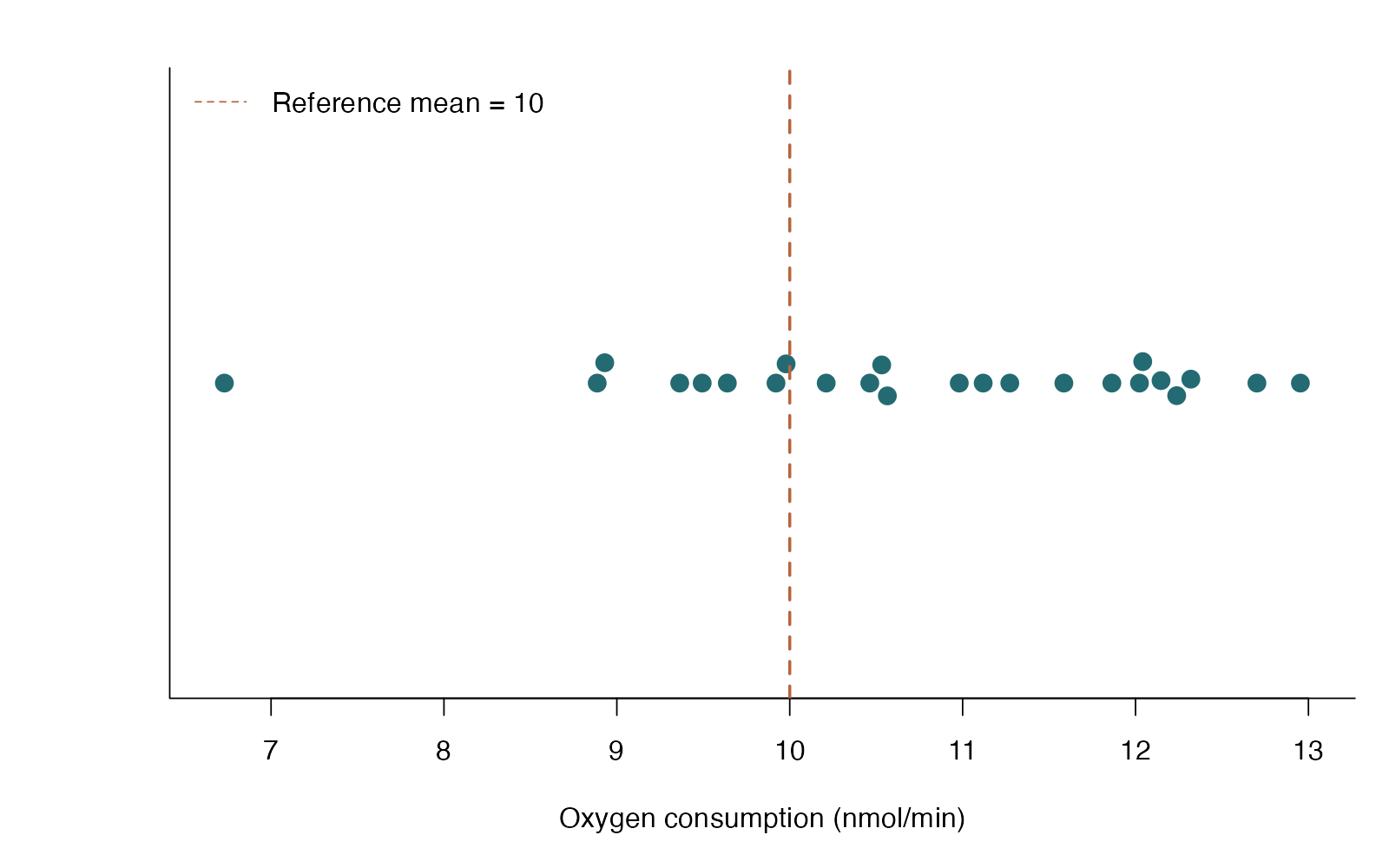
- Mean = 10.75 nmol/min; n = 24
- 95% CI for mean: 10.12 to 11.37
- t = 2.48; df = 23; p = 0.02107
Mean oxygen consumption was 10.75 nmol/min (95% CI 10.12 to 11.37); against the reference mean of 10, t(23) = 2.48, p = 0.02107. This tests a population mean, not whether every culture exceeds 10.
**Teaching point:** The reference must express the biological question; the test is about a population mean.
### Analysis code excerpt
```r
d <- read.csv("modules/one_sample_t/generated/data.csv")
fit <- t.test(d$oxygen, mu = 10,
alternative = "two.sided", conf.level = .95)
```
The full script supplies package loading and any additional preparation.
### Full printed R output
```text
One Sample t-test
data: d$oxygen
t = 2.4762, df = 23, p-value = 0.02107
alternative hypothesis: true mean is not equal to 10
95 percent confidence interval:
10.12316 11.37336
sample estimates:
mean of x
10.74826
```
### Recreate the observations
```r
output_dir <- "modules/one_sample_t/generated"
dir.create(output_dir, recursive = TRUE, showWarnings = FALSE)
set.seed(1101)
d <- data.frame(culture = 1:24,
oxygen = rnorm(24, mean = 10.8, sd = 1.5))
write.csv(d, file.path(output_dir, "data.csv"), row.names = FALSE)
```
Run the complete module from the course folder:
```sh
Rscript modules/one_sample_t/analysis.R modules/one_sample_t/generated
```
## Dataset 02: Pooled two-sample t test
Evolutionary biologists compare adult beetle body length from two rearing environments.
**Family:** Means · **Rows:** 56 · **Seed:** 1118
[Saved CSV](modules/pooled_t/generated/data.csv) · [Full runnable R script](modules/pooled_t/analysis.R) · [Full-size plot](modules/pooled_t/generated/plot.png)
**Generating truth:** The true Cool minus Warm mean difference is -0.7 mm, and the two population variances are both 0.4225 mm squared.
**Exact generating model:** 26 independent Cool beetles are Normal(10, 0.65 SD), and 30 independent Warm beetles are Normal(10.7, 0.65 SD).
**Scientific question:** Do mean body lengths differ between cool and warm environments?
**Null being tested / estimation target:** The two population means are equal.
**Design and independent unit:** Independent beetles in two rearing environments; a common population variance is a substantive model assumption.
### Columns
| Column | Meaning | Unit / type |
|---|---|---|
| environment | Independent rearing group | category |
| length_mm | Adult beetle body length | mm |
### Analysis from the saved dataset
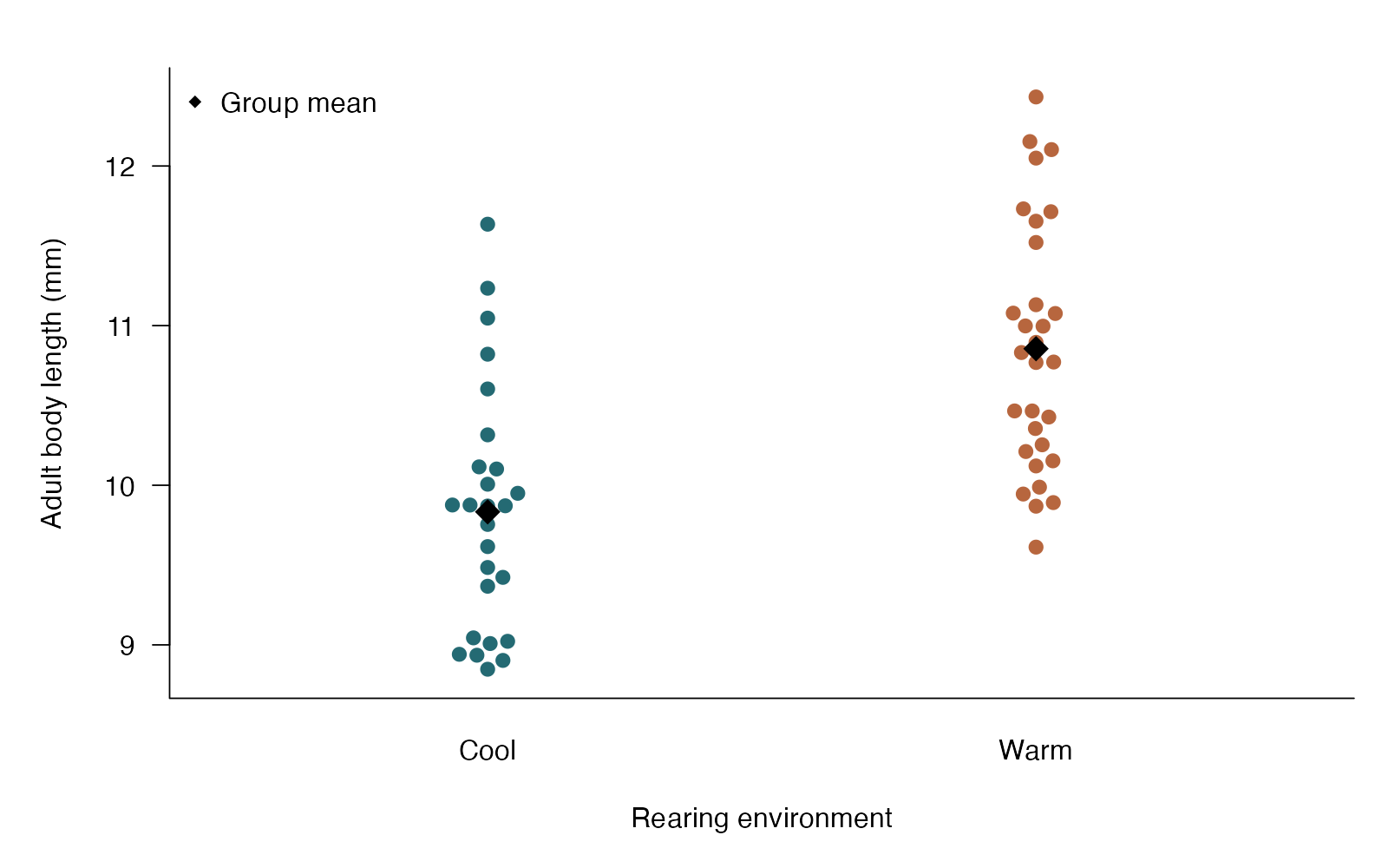
- Cool - Warm mean difference = -1.02 mm
- 95% CI: -1.44 to -0.61 mm
- Pooled t = -4.94; df = 54.00; p = 7.927e-06
Mean body length differed by -1.02 mm (Cool minus Warm; 95% CI -1.44 to -0.61). Pooled t = -4.94, df = 54.00, p = 7.927e-06. This analysis assumes equal population variances. Welch tests the same null without that assumption.
**Teaching point:** Pooled and Welch t tests share the mean-difference null; their variance assumptions differ.
### Analysis code excerpt
```r
d <- read.csv("modules/pooled_t/generated/data.csv")
d$environment <- factor(d$environment, levels = c("Cool", "Warm"))
fit <- t.test(length_mm ~ environment, data = d,
var.equal = TRUE, conf.level = .95)
difference <- mean(d$length_mm[d$environment == "Cool"]) -
mean(d$length_mm[d$environment == "Warm"])
```
The full script supplies package loading and any additional preparation.
### Full printed R output
```text
Two Sample t-test
data: length_mm by environment
t = -4.9399, df = 54, p-value = 7.927e-06
alternative hypothesis: true difference in means between group Cool and group Warm is not equal to 0
95 percent confidence interval:
-1.4367878 -0.6072203
sample estimates:
mean in group Cool mean in group Warm
9.833382 10.855386
```
### Recreate the observations
```r
output_dir <- "modules/pooled_t/generated"
dir.create(output_dir, recursive = TRUE, showWarnings = FALSE)
set.seed(1118)
d <- data.frame(environment = rep(c("Cool", "Warm"), c(26, 30)),
length_mm = c(rnorm(26, 10, .65), rnorm(30, 10.7, .65)))
write.csv(d, file.path(output_dir, "data.csv"), row.names = FALSE)
```
Run the complete module from the course folder:
```sh
Rscript modules/pooled_t/analysis.R modules/pooled_t/generated
```
## Dataset 03: Welch two-sample t test
Evolutionary biologists compare adult beetle body length from two rearing environments.
**Family:** Means · **Rows:** 56 · **Seed:** 1102
[Saved CSV](modules/welch_t/generated/data.csv) · [Full runnable R script](modules/welch_t/analysis.R) · [Full-size plot](modules/welch_t/generated/plot.png)
**Generating truth:** The true Cool minus Warm mean difference is -0.7 mm. Variances differ (0.4225 versus 1.3225 mm squared).
**Exact generating model:** 26 independent Cool lengths come from Normal(10, 0.65 SD), and 30 independent Warm lengths from Normal(10.7, 1.15 SD).
**Scientific question:** Do mean body lengths differ between cool and warm environments?
**Null being tested / estimation target:** The two population means are equal.
**Design and independent unit:** Independent beetles assigned to cool or warm rearing; each beetle measured once.
### Columns
| Column | Meaning | Unit / type |
|---|---|---|
| environment | Independent rearing group | category |
| length_mm | Adult beetle body length | mm |
### Analysis from the saved dataset
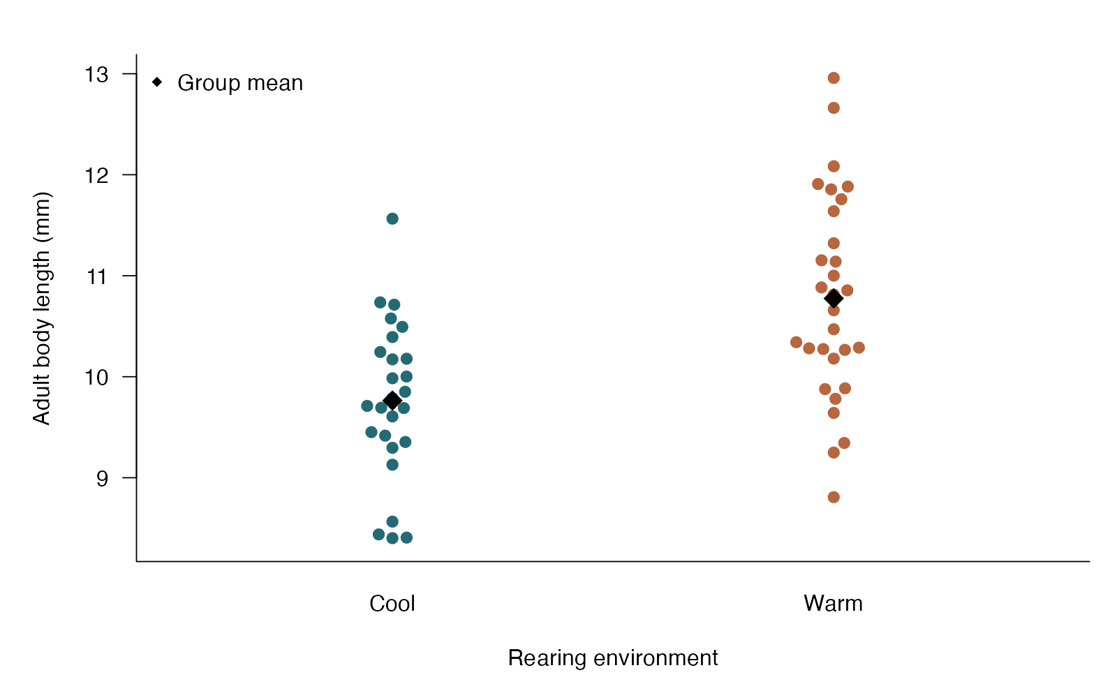
- Cool - Warm mean difference = -1.01 mm
- 95% CI: -1.49 to -0.53 mm
- Welch t = -4.21; df = 53.33; p = 9.973e-05
Mean body length differed by -1.01 mm (Cool minus Warm; 95% CI -1.49 to -0.53). Welch's t = -4.21, df = 53.33, p = 9.973e-05. Group ordering determines the sign; unequal group variances do not require switching to ranks.
**Teaching point:** Welch answers the equal-means question while allowing unequal group variances.
### Analysis code excerpt
```r
d <- read.csv("modules/welch_t/generated/data.csv")
d$environment <- factor(d$environment, levels = c("Cool", "Warm"))
fit <- t.test(length_mm ~ environment, data = d,
var.equal = FALSE, conf.level = .95)
difference <- mean(d$length_mm[d$environment == "Cool"]) -
mean(d$length_mm[d$environment == "Warm"])
```
The full script supplies package loading and any additional preparation.
### Full printed R output
```text
Welch Two Sample t-test
data: length_mm by environment
t = -4.2066, df = 53.33, p-value = 9.973e-05
alternative hypothesis: true difference in means between group Cool and group Warm is not equal to 0
95 percent confidence interval:
-1.4937879 -0.5292964
sample estimates:
mean in group Cool mean in group Warm
9.763781 10.775323
```
### Recreate the observations
```r
output_dir <- "modules/welch_t/generated"
dir.create(output_dir, recursive = TRUE, showWarnings = FALSE)
set.seed(1102)
d <- data.frame(environment = rep(c("Cool", "Warm"), c(26, 30)),
length_mm = c(rnorm(26, 10, .65), rnorm(30, 10.7, 1.15)))
write.csv(d, file.path(output_dir, "data.csv"), row.names = FALSE)
```
Run the complete module from the course folder:
```sh
Rscript modules/welch_t/analysis.R modules/welch_t/generated
```
## Dataset 04: Paired t test
Plant physiologists measure photosynthesis in the same leaves before and after heat stress.
**Family:** Means · **Rows:** 20 · **Seed:** 1103
[Saved CSV](modules/paired_t/generated/data.csv) · [Full runnable R script](modules/paired_t/analysis.R) · [Full-size plot](modules/paired_t/generated/plot.png)
**Generating truth:** The mean after-minus-before difference is -1.3 photosynthesis units, even if this sample provides limited evidence against zero.
**Exact generating model:** 20 independent baseline values come from Normal(18, 2.2 SD). Each after value is its own baseline plus an independent Normal(-1.3, 1.7 SD) change.
**Scientific question:** Is the mean within-plant change in photosynthesis zero?
**Null being tested / estimation target:** The population mean of after minus before differences is zero.
**Design and independent unit:** Twenty independent plants contribute one before/after pair each.
### Columns
| Column | Meaning | Unit / type |
|---|---|---|
| plant | Independent plant and pair identifier | none |
| before | Photosynthesis before heat | micromol CO2 / m2 / s |
| after | Photosynthesis after heat | micromol CO2 / m2 / s |
### Analysis from the saved dataset
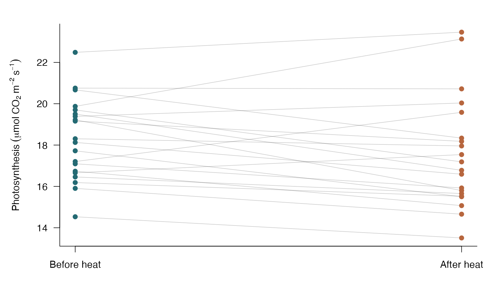
- Mean change (after - before) = -0.73
- 95% CI for mean change: -1.52 to 0.07
- Paired t = -1.91; df = 19; p = 0.07128
Photosynthesis changed by a mean of -0.73 units after heat stress (95% CI -1.52 to 0.07); paired t(19) = -1.91, p = 0.07128. Pairing makes the biological unit the plant and the analyzed response its change.
**Teaching point:** A large p-value does not make the simulated nonzero effect disappear; paired differences define the target.
### Analysis code excerpt
```r
d <- read.csv("modules/paired_t/generated/data.csv")
change <- d$after - d$before
fit <- t.test(d$after, d$before, paired = TRUE,
alternative = "two.sided")
```
The full script supplies package loading and any additional preparation.
### Full printed R output
```text
Paired t-test
data: d$after and d$before
t = -1.9105, df = 19, p-value = 0.07128
alternative hypothesis: true mean difference is not equal to 0
95 percent confidence interval:
-1.52238792 0.06942308
sample estimates:
mean difference
-0.7264824
```
### Recreate the observations
```r
output_dir <- "modules/paired_t/generated"
dir.create(output_dir, recursive = TRUE, showWarnings = FALSE)
set.seed(1103)
before <- rnorm(20, 18, 2.2)
after <- before + rnorm(20, -1.3, 1.7)
d <- data.frame(plant = 1:20, before = before, after = after)
write.csv(d, file.path(output_dir, "data.csv"), row.names = FALSE)
```
Run the complete module from the course folder:
```sh
Rscript modules/paired_t/analysis.R modules/paired_t/generated
```
## Dataset 05: F test of two variances
Evolutionary developmental biologists compare variation in wing length between two inbred fly lines.
**Family:** Variance and diagnostics · **Rows:** 60 · **Seed:** 1109
[Saved CSV](modules/f_variance/generated/data.csv) · [Full runnable R script](modules/f_variance/analysis.R) · [Full-size plot](modules/f_variance/generated/plot.png)
**Generating truth:** Population means are equal, but the true variance ratio A/B is 0.11 squared / 0.21 squared, approximately 0.274.
**Exact generating model:** 30 wing lengths per independent fly line come from normal distributions with shared mean 2.6 mm, SD 0.11 for Line A and SD 0.21 for Line B.
**Scientific question:** Is wing-length variance the same in the two fly lines?
**Null being tested / estimation target:** The population variance ratio (Line A / Line B) is 1.
**Design and independent unit:** Thirty independent flies per line are reared under a common environment.
### Columns
| Column | Meaning | Unit / type |
|---|---|---|
| line | Fly line | category |
| wing_mm | Wing length of one independent fly | mm |
### Analysis from the saved dataset
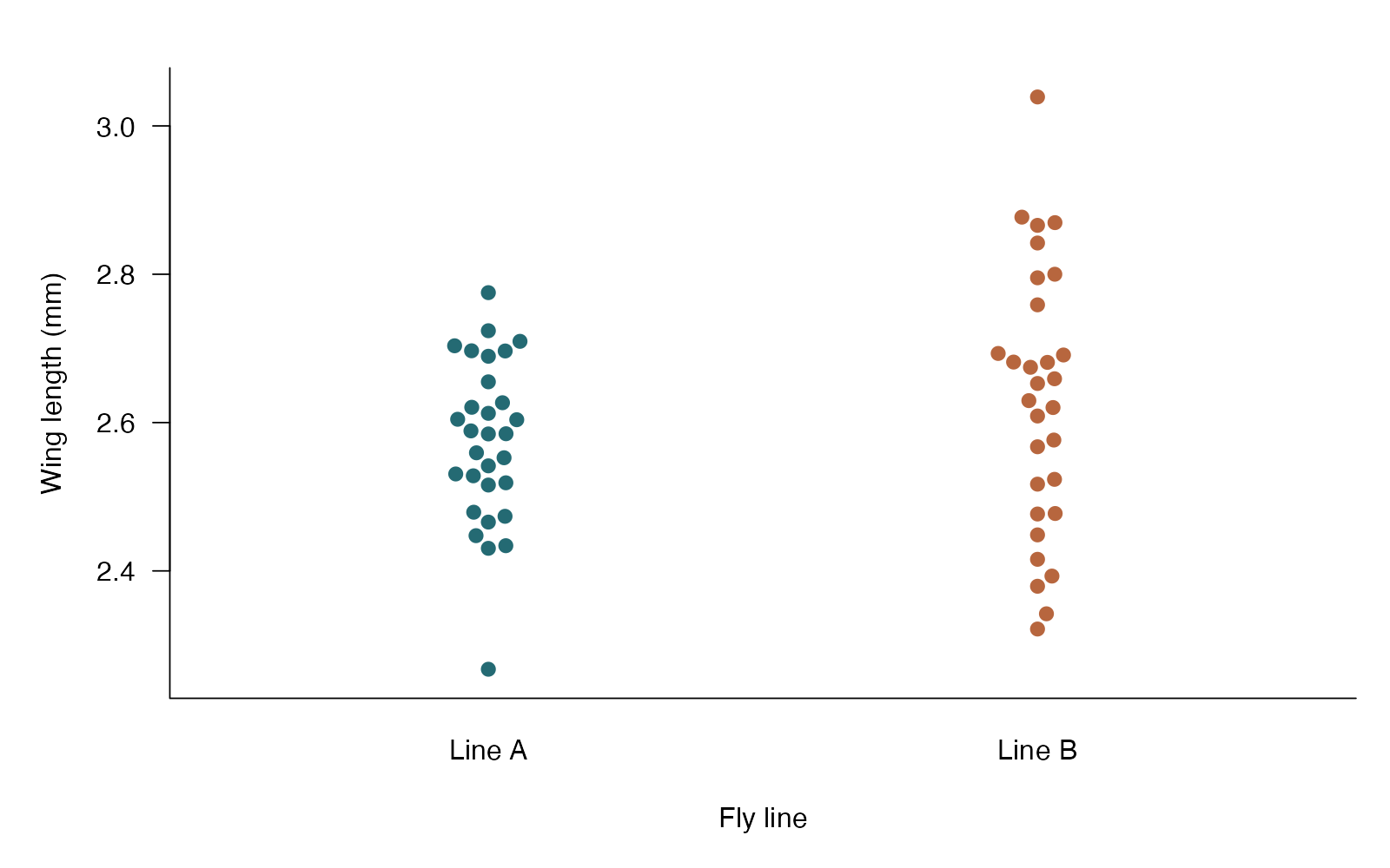
- Variance ratio (A / B) = 0.376
- 95% CI for variance ratio: 0.179 to 0.791
- F = 0.376; df = 29, 29; p = 0.01048
Wing-length variance in Line A was 0.376 times that in Line B (95% CI 0.179 to 0.791); F(29, 29) = 0.376, p = 0.01048. The target is variability, and this exact F reference relies strongly on normal populations.
**Teaching point:** A variance question can have a different answer from a mean question; the exact F test depends strongly on normality.
### Analysis code excerpt
```r
d <- read.csv("modules/f_variance/generated/data.csv")
d$line <- factor(d$line, levels = c("Line A", "Line B"))
fit <- var.test(wing_mm ~ line, data = d, ratio = 1,
alternative = "two.sided", conf.level = .95)
```
The full script supplies package loading and any additional preparation.
### Full printed R output
```text
F test to compare two variances
data: wing_mm by line
F = 0.37637, num df = 29, denom df = 29, p-value = 0.01048
alternative hypothesis: true ratio of variances is not equal to 1
95 percent confidence interval:
0.1791387 0.7907512
sample estimates:
ratio of variances
0.3763697
```
### Recreate the observations
```r
output_dir <- "modules/f_variance/generated"
dir.create(output_dir, recursive = TRUE, showWarnings = FALSE)
set.seed(1109)
d <- data.frame(line = rep(c("Line A", "Line B"), each = 30),
wing_mm = c(rnorm(30, 2.6, .11), rnorm(30, 2.6, .21)))
write.csv(d, file.path(output_dir, "data.csv"), row.names = FALSE)
```
Run the complete module from the course folder:
```sh
Rscript modules/f_variance/analysis.R modules/f_variance/generated
```
## Dataset 06: Levene and Brown–Forsythe tests
Microbiologists compare the variability of colony diameters across three nutrient media.
**Family:** Variance and diagnostics · **Rows:** 84 · **Seed:** 1110
[Saved CSV](modules/levene/generated/data.csv) · [Full runnable R script](modules/levene/analysis.R) · [Full-size plot](modules/levene/generated/plot.png)
**Generating truth:** Group geometric means are 4 mm, but variances differ. Arithmetic means also vary slightly because log-normal means depend on log-scale spread.
**Exact generating model:** 28 independently cultured colonies per medium have log-normal diameters. All have meanlog log(4); log-scale SD is 0.12, 0.20, or 0.35 for Low, Medium, and High medium.
**Scientific question:** Do population variances differ among nutrient media?
**Null being tested / estimation target:** The groups have equal variances; the test compares absolute deviations from their group centers.
**Design and independent unit:** Independent colonies are grown in separately inoculated culture wells; one colony measured per well.
### Columns
| Column | Meaning | Unit / type |
|---|---|---|
| medium | Nutrient medium | category |
| diameter_mm | Diameter of a colony from one independent well | mm |
### Analysis from the saved dataset
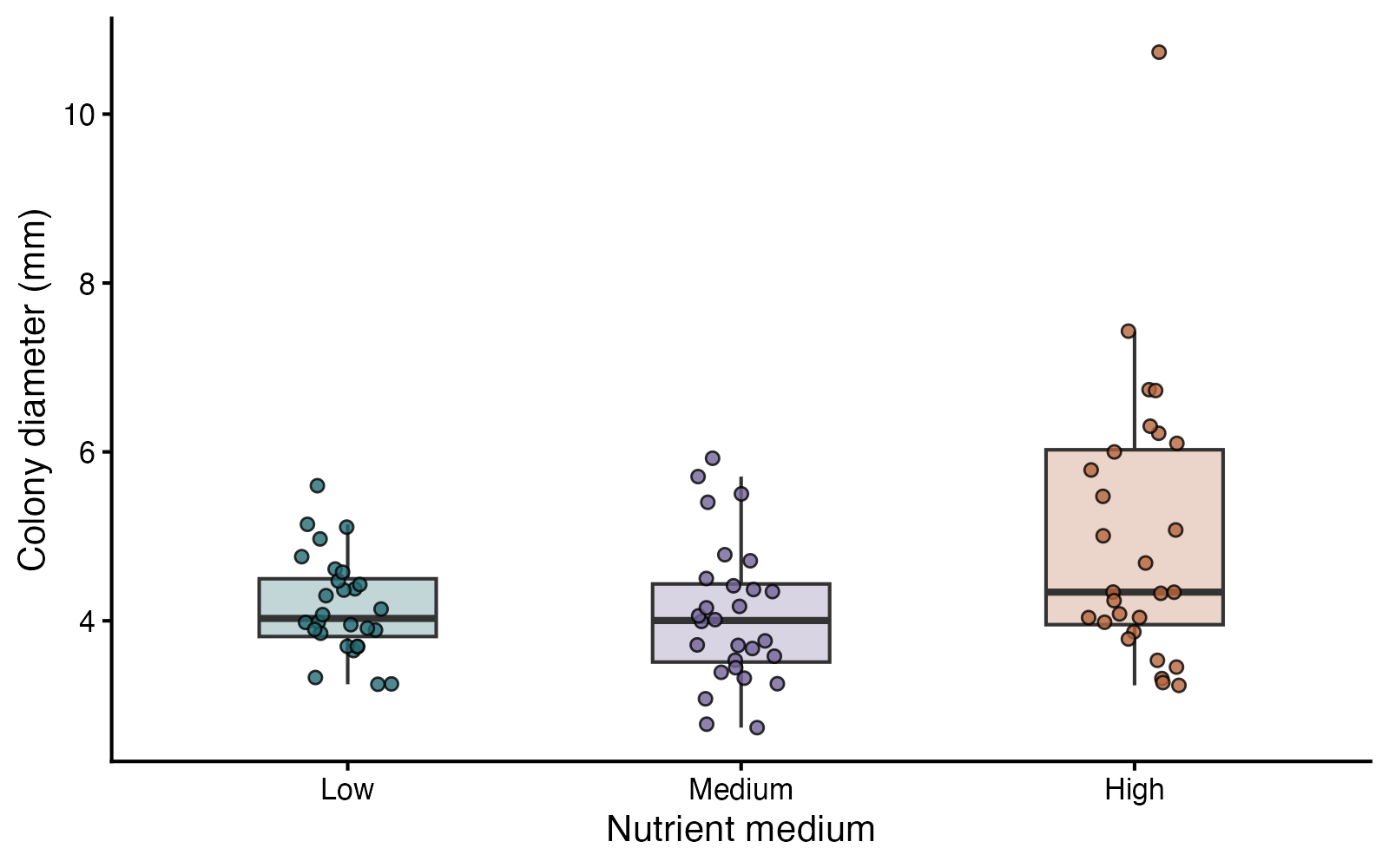
- Brown–Forsythe F = 5.55; df = 2, 81; p = 0.005524
- Original Levene F = 9.72; p = 0.0001645
- Observed group SDs: Low 0.59; Medium 0.84; High 1.64
The median-centered Brown–Forsythe comparison gave F(2, 81) = 5.55, p = 0.005524. Inspect the distributions as well as the p-value: the procedure compares absolute deviations, which can reflect both spread and shape.
**Teaching point:** Median-centered Brown–Forsythe reduces sensitivity to long tails; it is not a required gate before Welch mean comparisons.
### Analysis code excerpt
```r
d <- read.csv("modules/levene/generated/data.csv")
d$medium <- factor(d$medium, levels = c("Low", "Medium", "High"))
brown_forsythe <- leveneTest(diameter_mm ~ medium, data = d,
center = median)
original_levene <- leveneTest(diameter_mm ~ medium, data = d,
center = mean)
```
The full script supplies package loading and any additional preparation.
### Full printed R output
```text
Levene's Test for Homogeneity of Variance (center = median)
Df F value Pr(>F)
group 2 5.5471 0.005524 **
81
---
Signif. codes: 0 ‘***’ 0.001 ‘**’ 0.01 ‘*’ 0.05 ‘.’ 0.1 ‘ ’ 1
Levene's Test for Homogeneity of Variance (center = mean)
Df F value Pr(>F)
group 2 9.7209 0.0001645 ***
81
---
Signif. codes: 0 ‘***’ 0.001 ‘**’ 0.01 ‘*’ 0.05 ‘.’ 0.1 ‘ ’ 1
```
### Recreate the observations
```r
output_dir <- "modules/levene/generated"
dir.create(output_dir, recursive = TRUE, showWarnings = FALSE)
set.seed(1110)
d <- data.frame(medium = rep(c("Low", "Medium", "High"), each = 28),
diameter_mm = c(rlnorm(28, log(4), .12),
rlnorm(28, log(4), .20), rlnorm(28, log(4), .35)))
write.csv(d, file.path(output_dir, "data.csv"), row.names = FALSE)
```
Run the complete module from the course folder:
```sh
Rscript modules/levene/analysis.R modules/levene/generated
```
## Dataset 07: Shapiro–Wilk and graphical checks
Cell biologists examine the distribution of time to lysis among independent cultured cells.
**Family:** Variance and diagnostics · **Rows:** 36 · **Seed:** 1111
[Saved CSV](modules/shapiro/generated/data.csv) · [Full runnable R script](modules/shapiro/analysis.R) · [Full-size plot](modules/shapiro/generated/plot.png)
**Generating truth:** The population is log-normal and positively skewed, not normal. The population geometric mean is 45 minutes.
**Exact generating model:** 36 independent lysis times follow a log-normal distribution with meanlog log(45) and log-scale SD 0.5.
**Scientific question:** Is a normal model a reasonable working description of these lysis times?
**Null being tested / estimation target:** The independent observations come from a normal distribution.
**Design and independent unit:** One lysis time for each independently treated culture; use a diagnostic to investigate shape.
### Columns
| Column | Meaning | Unit / type |
|---|---|---|
| culture | Independent culture identifier | none |
| lysis_minutes | Time until lysis | minutes |
### Analysis from the saved dataset
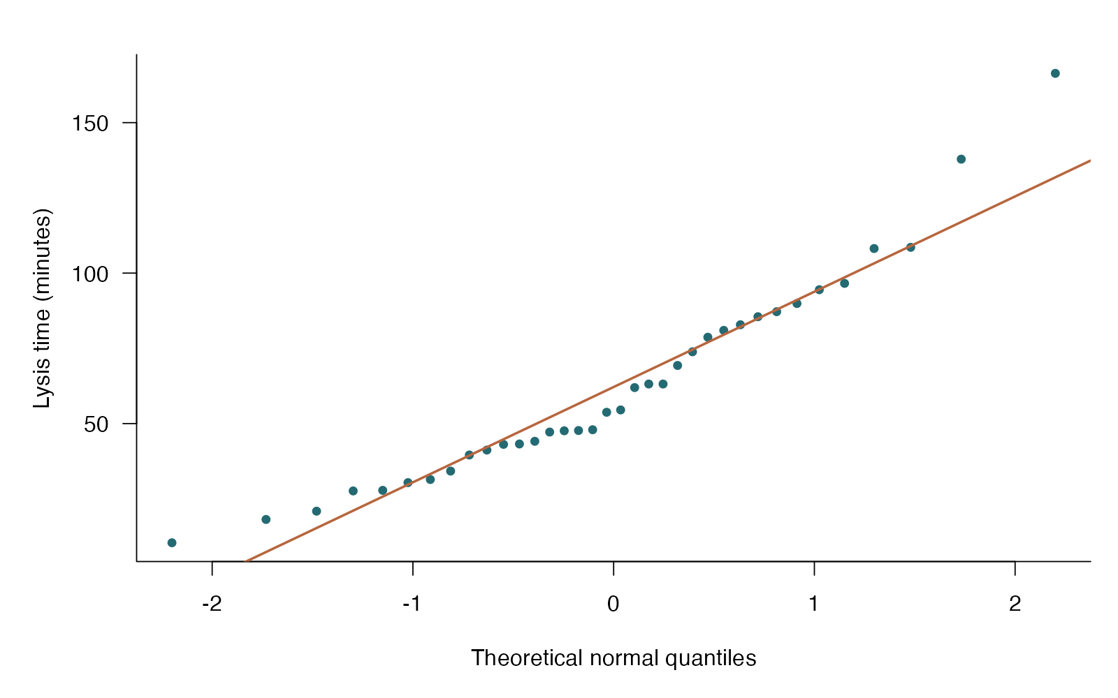
- Shapiro–Wilk W = 0.937; p = 0.04064; n = 36
- Curvature in the Q–Q plot indicates a shape mismatch.
- A nonsignificant result would not establish normality.
For the 36 lysis times, Shapiro–Wilk W = 0.937, p = 0.04064. Use the Q–Q plot to understand the mismatch; this diagnostic alone does not choose the scientific test or show that a mean comparison is invalid.
**Teaching point:** A diagnostic explains how a working model misses the data; its p-value should not automatically select the scientific analysis.
### Analysis code excerpt
```r
d <- read.csv("modules/shapiro/generated/data.csv")
fit <- shapiro.test(d$lysis_minutes)
```
The full script supplies package loading and any additional preparation.
### Full printed R output
```text
Shapiro-Wilk normality test
data: d$lysis_minutes
W = 0.93687, p-value = 0.04064
```
### Recreate the observations
```r
output_dir <- "modules/shapiro/generated"
dir.create(output_dir, recursive = TRUE, showWarnings = FALSE)
set.seed(1111)
d <- data.frame(culture = 1:36,
lysis_minutes = rlnorm(36, log(45), .5))
write.csv(d, file.path(output_dir, "data.csv"), row.names = FALSE)
```
Run the complete module from the course folder:
```sh
Rscript modules/shapiro/analysis.R modules/shapiro/generated
```
## Dataset 08: Sign test
Behavioral biologists record the change in refuge-use time after a predator cue.
**Family:** Nonparametric alternatives · **Rows:** 30 · **Seed:** 1104
[Saved CSV](modules/sign_test/generated/data.csv) · [Full runnable R script](modules/sign_test/analysis.R) · [Full-size plot](modules/sign_test/generated/plot.png)
**Generating truth:** Positive changes are more likely than negative changes. The unrounded mean is 4 seconds, but the sign test is about direction rather than that mean.
**Exact generating model:** 30 independent changes are Gamma(shape 1.4, scale 5) minus 3 seconds, rounded to 0.1 seconds. Exact zeros, if present, are excluded from the sign comparison.
**Scientific question:** Is an increase just as likely as a decrease in refuge-use time?
**Null being tested / estimation target:** Among nonzero changes, positive and negative changes are equally likely; for continuous differences, the median is zero.
**Design and independent unit:** Each independent fish is measured twice; the changes are skewed.
### Columns
| Column | Meaning | Unit / type |
|---|---|---|
| fish | Independent fish and pair identifier | none |
| change_seconds | After-minus-before refuge-use time | seconds |
### Analysis from the saved dataset
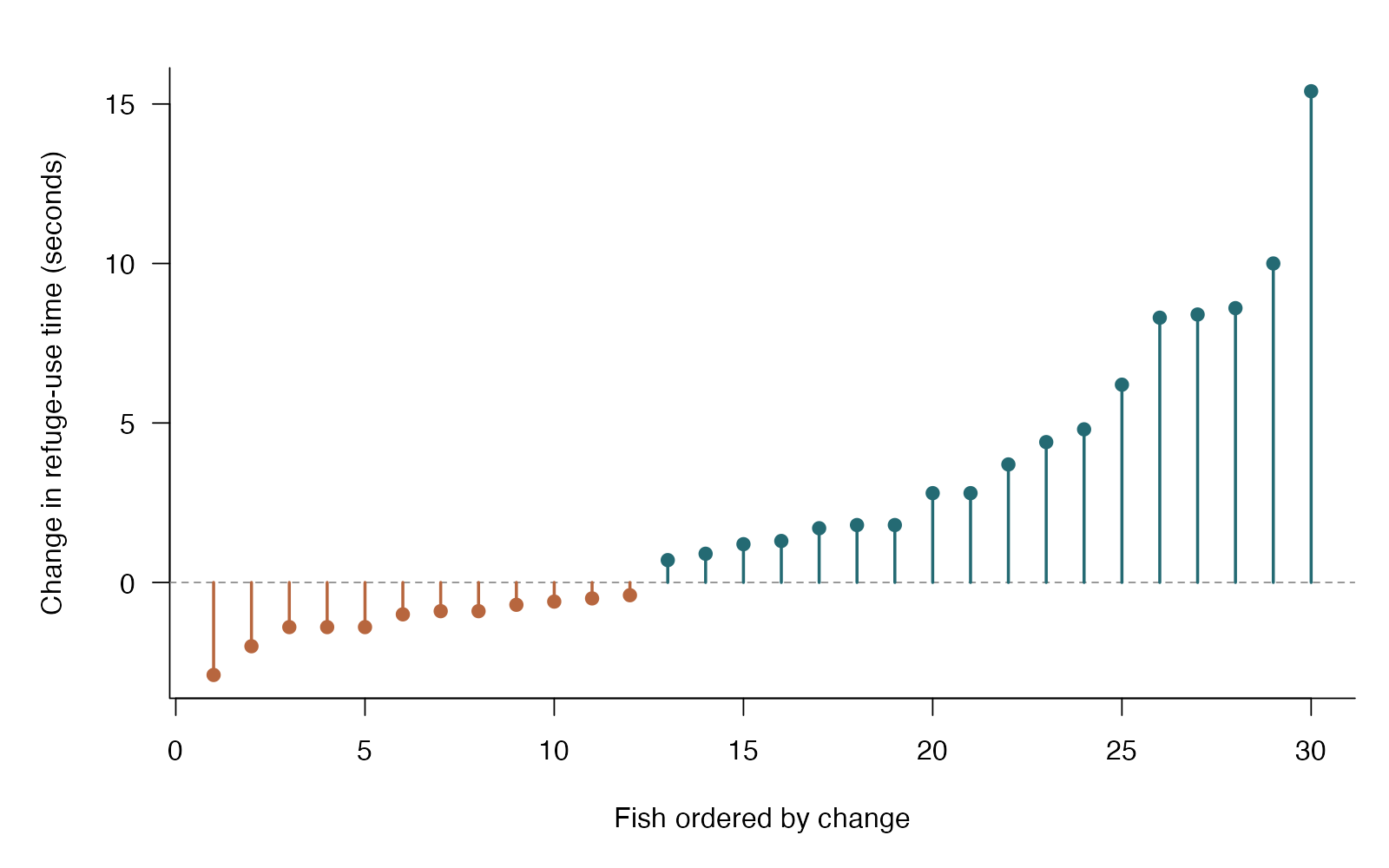
- Positive changes: 18 of 30 nonzero differences
- Zero changes excluded: 0
- Median observed change = 1.25 seconds
- 95% CI for positive-change probability: 0.41 to 0.77
- Exact two-sided p = 0.3616
18 of 30 nonzero changes were positive (exact sign-test p = 0.3616; 95% CI for the positive-change probability 0.41 to 0.77). The test asks about direction, not mean change; 0 exact zero differences were excluded.
**Teaching point:** A sign test handles asymmetric differences by asking about the probability of a positive change.
### Analysis code excerpt
```r
d <- read.csv("modules/sign_test/generated/data.csv")
nonzero <- d$change_seconds[d$change_seconds != 0]
positive <- sum(nonzero > 0)
fit <- binom.test(positive, length(nonzero), p = .5,
alternative = "two.sided")
```
The full script supplies package loading and any additional preparation.
### Full printed R output
```text
Exact binomial test
data: positive and length(nonzero)
number of successes = 18, number of trials = 30, p-value = 0.3616
alternative hypothesis: true probability of success is not equal to 0.5
95 percent confidence interval:
0.4060349 0.7734424
sample estimates:
probability of success
0.6
```
### Recreate the observations
```r
output_dir <- "modules/sign_test/generated"
dir.create(output_dir, recursive = TRUE, showWarnings = FALSE)
set.seed(1104)
change <- rgamma(30, shape = 1.4, scale = 5) - 3
d <- data.frame(fish = 1:30, change_seconds = round(change, 1))
write.csv(d, file.path(output_dir, "data.csv"), row.names = FALSE)
```
Run the complete module from the course folder:
```sh
Rscript modules/sign_test/analysis.R modules/sign_test/generated
```
## Dataset 09: Wilcoxon signed-rank test
Microbiologists compare log bacterial density before and after a treatment in matched cultures.
**Family:** Nonparametric alternatives · **Rows:** 28 · **Seed:** 1105
[Saved CSV](modules/signed_rank/generated/data.csv) · [Full runnable R script](modules/signed_rank/analysis.R) · [Full-size plot](modules/signed_rank/generated/plot.png)
**Generating truth:** The symmetric difference distribution is centered at +0.28 log10 units; its zero-center null is false.
**Exact generating model:** 28 baselines come from Normal(6, 0.4 SD). Paired changes equal 0.28 + 0.28 times a Student t variable with 4 degrees of freedom; after equals before plus change.
**Scientific question:** Is the distribution of within-culture changes centered at zero?
**Null being tested / estimation target:** The difference distribution is symmetric about zero.
**Design and independent unit:** Each independent culture contributes one difference; occasional large differences make ranks useful.
### Columns
| Column | Meaning | Unit / type |
|---|---|---|
| culture | Independent culture and pair identifier | none |
| before | Log10 bacterial density before treatment | log10 CFU/mL |
| after | Log10 bacterial density after treatment | log10 CFU/mL |
### Analysis from the saved dataset
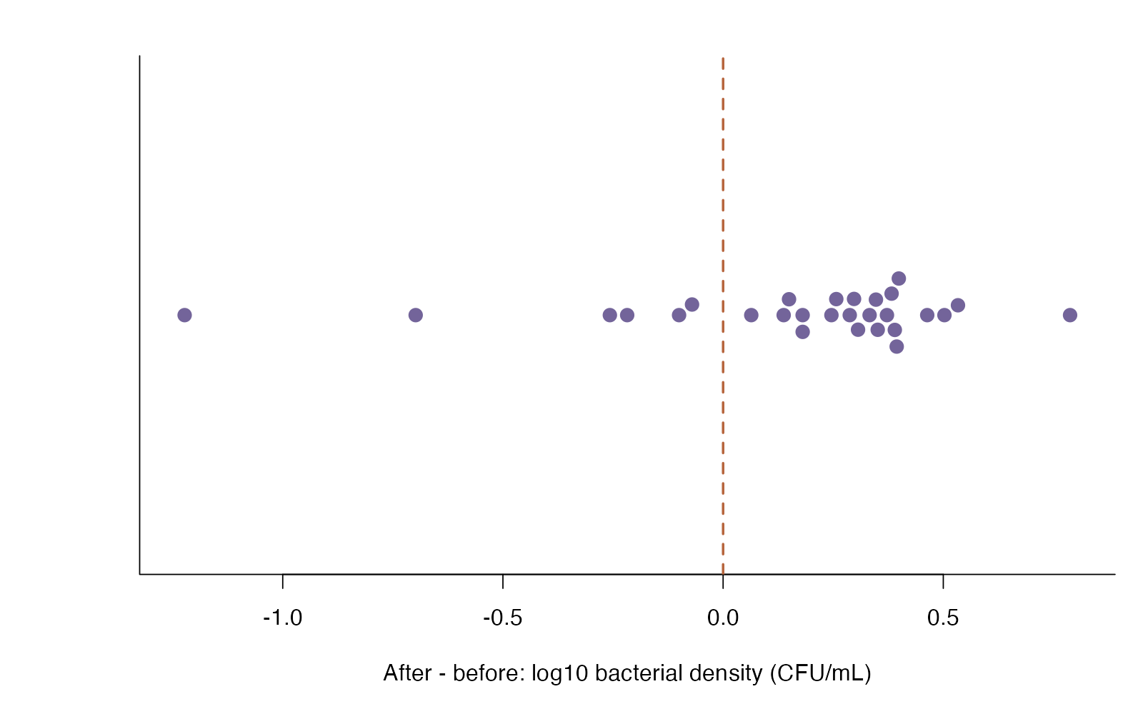
- Pseudomedian change estimate = 0.249
- 95% CI: 0.094 to 0.341
- V = 328.0; p = 0.004582
The estimated pseudomedian log10 density change was 0.249 (95% CI 0.094 to 0.341); signed-rank V = 328.0, p = 0.004582. Under a symmetric location-shift model this describes the common center of the differences; the procedure does not generally test a mean.
**Teaching point:** Signed-rank is useful for symmetric heavy-tailed differences; sign is the simpler alternative when symmetry is doubtful.
### Analysis code excerpt
```r
d <- read.csv("modules/signed_rank/generated/data.csv")
change <- d$after - d$before
fit <- wilcox.test(d$after, d$before, paired = TRUE,
exact = FALSE, conf.int = TRUE)
```
The full script supplies package loading and any additional preparation.
### Full printed R output
```text
Wilcoxon signed rank test with continuity correction
data: d$after and d$before
V = 328, p-value = 0.004582
alternative hypothesis: true location shift is not equal to 0
95 percent confidence interval:
0.09375924 0.34088634
sample estimates:
(pseudo)median
0.2486103
```
### Recreate the observations
```r
output_dir <- "modules/signed_rank/generated"
dir.create(output_dir, recursive = TRUE, showWarnings = FALSE)
set.seed(1105)
before <- rnorm(28, 6, .4)
after <- before + .28 + .28 * rt(28, df = 4)
d <- data.frame(culture = 1:28, before = before, after = after)
write.csv(d, file.path(output_dir, "data.csv"), row.names = FALSE)
```
Run the complete module from the course folder:
```sh
Rscript modules/signed_rank/analysis.R modules/signed_rank/generated
```
## Dataset 10: Wilcoxon rank-sum test
Ecologists compare parasite burdens among fish from two independent lakes.
**Family:** Nonparametric alternatives · **Rows:** 64 · **Seed:** 1106
[Saved CSV](modules/rank_sum/generated/data.csv) · [Full runnable R script](modules/rank_sum/analysis.R) · [Full-size plot](modules/rank_sum/generated/plot.png)
**Generating truth:** The lake distributions differ, including their mean and spread. The same-distribution null is false; there is not a simple equal-shape location shift.
**Exact generating model:** 32 independent fish per lake have negative-binomial parasite counts. Clear has mean 5 and Reedy mean 10, both with size parameter 1.5; variances are mean + mean squared / 1.5.
**Scientific question:** Do parasite-burden distributions differ between the two lakes?
**Null being tested / estimation target:** The two groups have the same response distribution.
**Design and independent unit:** Each fish is sampled once; counts are strongly skewed and tied.
### Columns
| Column | Meaning | Unit / type |
|---|---|---|
| lake | Lake of independently sampled fish | category |
| parasites | Parasite burden of one fish | count |
### Analysis from the saved dataset
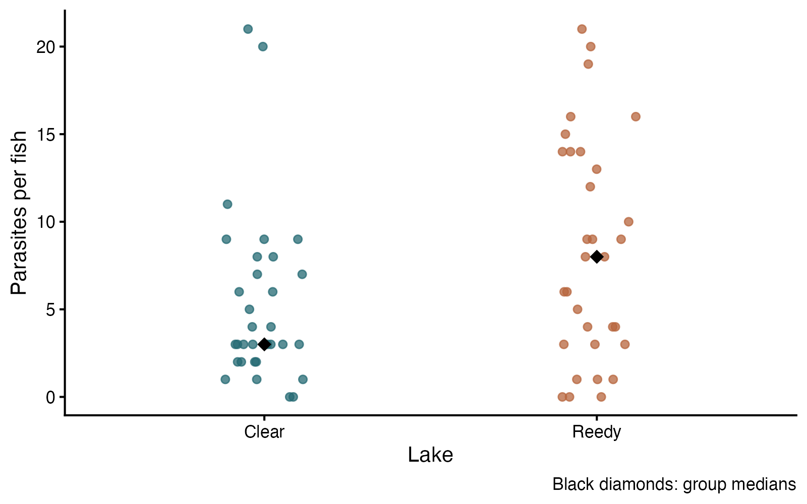
- Observed medians: Clear 3.0; Reedy 8.0 parasites
- W = 362.5; asymptotic p = 0.04452
- Medians describe these data; the general null concerns distributions.
Parasite burdens had observed medians 3.0 (Clear) and 8.0 (Reedy). The rank-sum comparison gave W = 362.5, p = 0.04452. This is evidence about the distributions; calling it a median test requires additional shape assumptions.
**Teaching point:** A rank-sum result can reflect distributional differences; the mean-count question also has a direct count-model route.
### Analysis code excerpt
```r
d <- read.csv("modules/rank_sum/generated/data.csv")
fit <- wilcox.test(parasites ~ lake, data = d,
exact = FALSE, correct = TRUE)
```
The full script supplies package loading and any additional preparation.
### Full printed R output
```text
Wilcoxon rank sum test with continuity correction
data: parasites by lake
W = 362.5, p-value = 0.04452
alternative hypothesis: true location shift is not equal to 0
```
### Recreate the observations
```r
output_dir <- "modules/rank_sum/generated"
dir.create(output_dir, recursive = TRUE, showWarnings = FALSE)
set.seed(1106)
d <- data.frame(lake = rep(c("Clear", "Reedy"), each = 32),
parasites = c(rnbinom(32, mu = 5, size = 1.5),
rnbinom(32, mu = 10, size = 1.5)))
write.csv(d, file.path(output_dir, "data.csv"), row.names = FALSE)
```
Run the complete module from the course folder:
```sh
Rscript modules/rank_sum/analysis.R modules/rank_sum/generated
```
## Dataset 11: One-way ANOVA
Ecologists compare seedling biomass under three independent soil treatments.
**Family:** ANOVA · **Rows:** 75 · **Seed:** 1117
[Saved CSV](modules/one_way_anova/generated/data.csv) · [Full runnable R script](modules/one_way_anova/analysis.R) · [Full-size plot](modules/one_way_anova/generated/plot.png)
**Generating truth:** The equal-means null is false. All three populations share variance 0.85 squared; Loam minus Sand is truly 0.9 g.
**Exact generating model:** 25 independent biomass values per soil come from normal distributions: Sand mean 4.5, Loam mean 5.4, Clay mean 5.1 g; every group has SD 0.85 g.
**Scientific question:** Are mean seedling biomasses equal across the three soils?
**Null being tested / estimation target:** All soil-treatment population means are equal.
**Design and independent unit:** Twenty-five independently assigned pots per soil treatment; one biomass value per pot.
### Columns
| Column | Meaning | Unit / type |
|---|---|---|
| soil | Assigned soil treatment | category |
| biomass_g | Seedling biomass from one independent pot | g |
### Analysis from the saved dataset
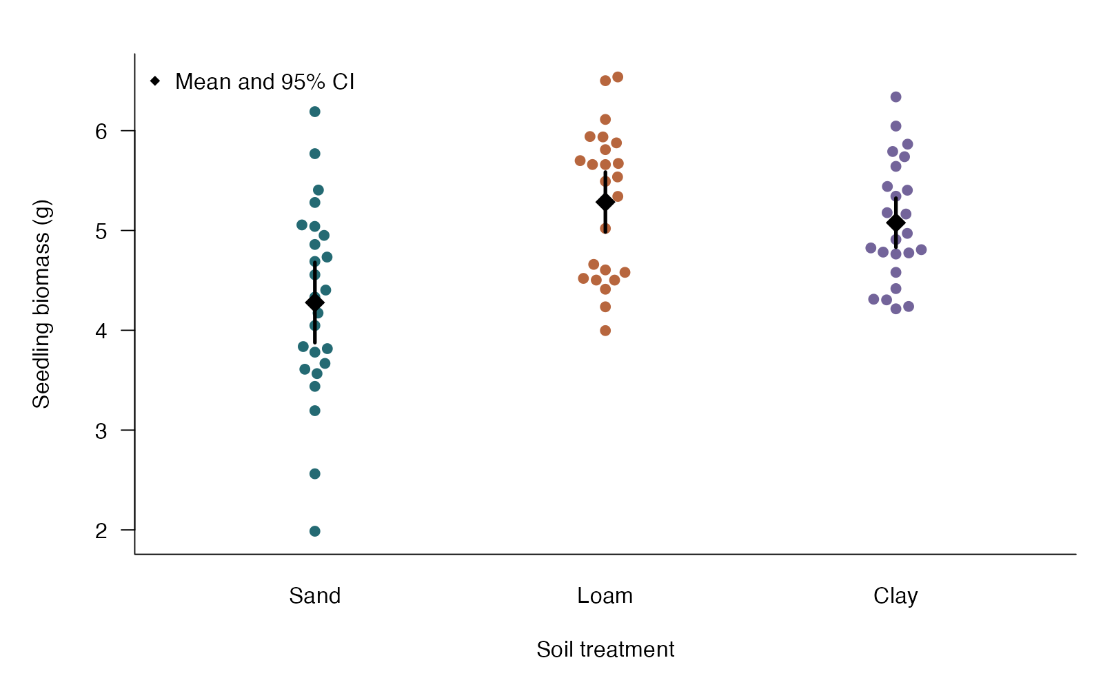
- Ordinary ANOVA F(2, 72) = 11.59; p = 4.335e-05
- Welch ANOVA F = 8.89; denominator df = 46.37; p = 0.0005408
- Observed means (g): Sand 4.28; Loam 5.28; Clay 5.08
- Neither omnibus test identifies a specific differing pair.
Mean seedling biomass was compared across soils with ordinary ANOVA: F(2, 72) = 11.59, p = 4.335e-05. Welch ANOVA, which relaxes equal variances, gave p = 0.0005408. Use a planned contrast or adjusted pairwise comparisons to answer which means differ.
**Teaching point:** The omnibus equal-means question differs from a scientific question about one particular contrast.
### Analysis code excerpt
```r
d <- read.csv("modules/one_way_anova/generated/data.csv")
d$soil <- factor(d$soil, levels = c("Sand", "Loam", "Clay"))
fit <- aov(biomass_g ~ soil, data = d)
anova_table <- summary(fit)[[1]]
welch <- oneway.test(biomass_g ~ soil, data = d,
var.equal = FALSE)
```
The full script supplies package loading and any additional preparation.
### Full printed R output
```text
Df Sum Sq Mean Sq F value Pr(>F)
soil 2 14.14 7.068 11.59 4.34e-05 ***
Residuals 72 43.92 0.610
---
Signif. codes: 0 ‘***’ 0.001 ‘**’ 0.01 ‘*’ 0.05 ‘.’ 0.1 ‘ ’ 1
One-way analysis of means (not assuming equal variances)
data: biomass_g and soil
F = 8.8862, num df = 2.000, denom df = 46.371, p-value = 0.0005408
```
### Recreate the observations
```r
output_dir <- "modules/one_way_anova/generated"
dir.create(output_dir, recursive = TRUE, showWarnings = FALSE)
set.seed(1117)
d <- data.frame(soil = rep(c("Sand", "Loam", "Clay"), each = 25),
biomass_g = c(rnorm(25, 4.5, .85), rnorm(25, 5.4, .85),
rnorm(25, 5.1, .85)))
write.csv(d, file.path(output_dir, "data.csv"), row.names = FALSE)
```
Run the complete module from the course folder:
```sh
Rscript modules/one_way_anova/analysis.R modules/one_way_anova/generated
```
## Dataset 12: Welch one-way ANOVA
Ecologists compare seedling biomass under three independent soil treatments.
**Family:** ANOVA · **Rows:** 78 · **Seed:** 1119
[Saved CSV](modules/welch_anova/generated/data.csv) · [Full runnable R script](modules/welch_anova/analysis.R) · [Full-size plot](modules/welch_anova/generated/plot.png)
**Generating truth:** The true means differ, and variances differ (0.36, 1.21, and 2.25 g squared). Welch addresses the equal-means null without a shared variance.
**Exact generating model:** Independent soil groups have different sample sizes and normal biomass distributions: Sand n=20, mean 4.5, SD 0.6; Loam n=26, mean 5.4, SD 1.1; Clay n=32, mean 5.1, SD 1.5.
**Scientific question:** Are mean seedling biomasses equal across the three soils?
**Null being tested / estimation target:** All soil-treatment population means are equal.
**Design and independent unit:** Independent pots in three soil treatments; sample sizes and group variances differ.
### Columns
| Column | Meaning | Unit / type |
|---|---|---|
| soil | Assigned soil treatment | category |
| biomass_g | Seedling biomass from one independent pot | g |
### Analysis from the saved dataset
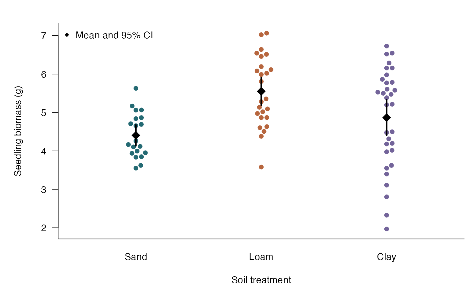
- Welch ANOVA F = 13.65; df = 2, 49.85; p = 1.873e-05
- Group sample sizes: Sand 20; Loam 26; Clay 32
- Observed means (g): Sand 4.4; Loam 5.55; Clay 4.87
- Unequal variance is modeled; the omnibus test does not select a pair.
Welch ANOVA compared mean biomass across soils while allowing unequal variances: F(2, 49.85) = 13.65, p = 1.873e-05. This answers the same equal-means question as ordinary ANOVA; a specific pair requires an appropriate adjusted follow-up.
**Teaching point:** Unequal variances have a parametric solution that preserves the scientific question about means.
### Analysis code excerpt
```r
d <- read.csv("modules/welch_anova/generated/data.csv")
d$soil <- factor(d$soil, levels = c("Sand", "Loam", "Clay"))
fit <- oneway.test(biomass_g ~ soil, data = d,
var.equal = FALSE)
```
The full script supplies package loading and any additional preparation.
### Full printed R output
```text
One-way analysis of means (not assuming equal variances)
data: biomass_g and soil
F = 13.65, num df = 2.000, denom df = 49.854, p-value = 1.873e-05
```
### Recreate the observations
```r
output_dir <- "modules/welch_anova/generated"
dir.create(output_dir, recursive = TRUE, showWarnings = FALSE)
set.seed(1119)
d <- data.frame(soil = rep(c("Sand", "Loam", "Clay"), c(20, 26, 32)),
biomass_g = c(rnorm(20, 4.5, .6), rnorm(26, 5.4, 1.1),
rnorm(32, 5.1, 1.5)))
write.csv(d, file.path(output_dir, "data.csv"), row.names = FALSE)
```
Run the complete module from the course folder:
```sh
Rscript modules/welch_anova/analysis.R modules/welch_anova/generated
```
## Dataset 13: Kruskal–Wallis test
Plant pathologists score leaf damage in three independently assigned pathogen treatments.
**Family:** Nonparametric alternatives · **Rows:** 72 · **Seed:** 1107
[Saved CSV](modules/kruskal_wallis/generated/data.csv) · [Full runnable R script](modules/kruskal_wallis/analysis.R) · [Full-size plot](modules/kruskal_wallis/generated/plot.png)
**Generating truth:** The score distributions differ across all three generating probabilities; expected scores are 2.0, 3.2, and 4.64. The equal-distributions null is false.
**Exact generating model:** 24 independent plants per group receive binomial damage scores with 8 trials and probabilities 0.25 (Control), 0.40 (Strain A), and 0.58 (Strain B). The score is used as an ordered severity scale.
**Scientific question:** Do damage-score distributions differ among pathogen treatments?
**Null being tested / estimation target:** All groups share the same response distribution.
**Design and independent unit:** Twenty-four independent plants per treatment; ordinal damage scores run from 0 to 8.
### Columns
| Column | Meaning | Unit / type |
|---|---|---|
| treatment | Assigned pathogen treatment | category |
| damage | Ordered leaf-damage score | score 0 to 8 |
### Analysis from the saved dataset
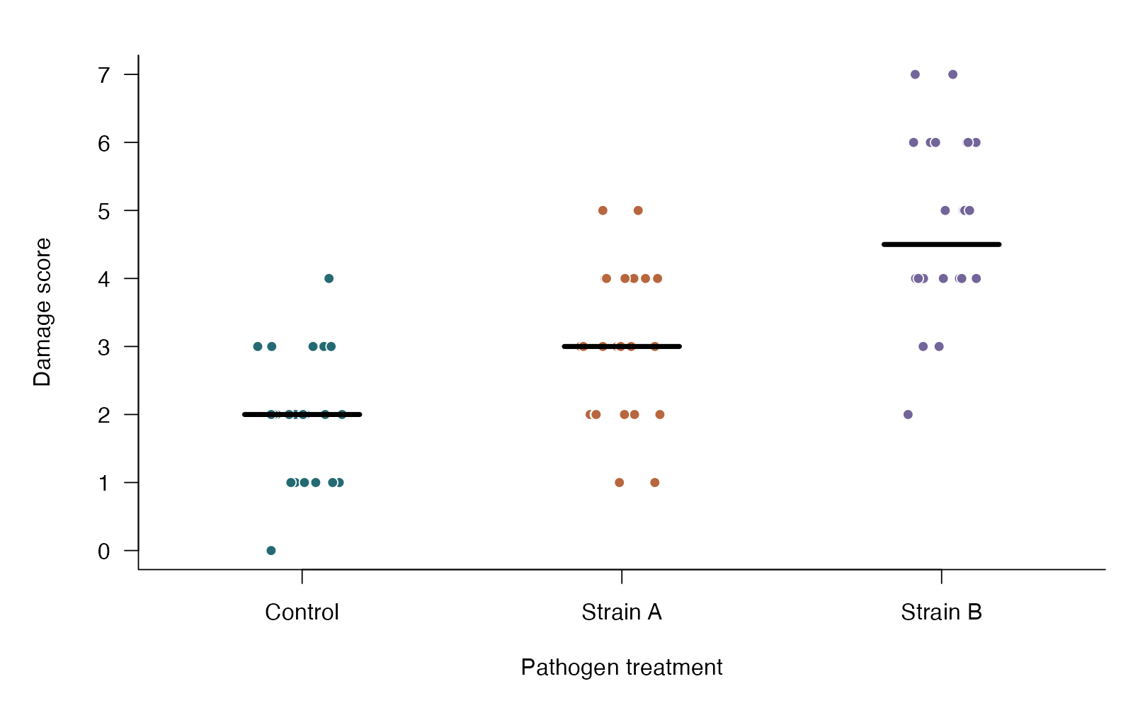
- Kruskal–Wallis chi-square = 35.75; df = 2; p = 1.73e-08
- Observed medians: Control 2; Strain A 3; Strain B 4.5
- The omnibus result does not identify which pairs differ.
Damage-score distributions were compared using Kruskal–Wallis: chi-square(2) = 35.75, p = 1.73e-08. An omnibus result concerns at least one group difference; it does not identify a particular pair or generally establish different medians.
**Teaching point:** An omnibus rank result identifies a group-level difference without choosing a pair.
### Analysis code excerpt
```r
d <- read.csv("modules/kruskal_wallis/generated/data.csv")
d$treatment <- factor(d$treatment, levels = c("Control", "Strain A", "Strain B"))
fit <- kruskal.test(damage ~ treatment, data = d)
```
The full script supplies package loading and any additional preparation.
### Full printed R output
```text
Kruskal-Wallis rank sum test
data: damage by treatment
Kruskal-Wallis chi-squared = 35.745, df = 2, p-value = 1.73e-08
```
### Recreate the observations
```r
output_dir <- "modules/kruskal_wallis/generated"
dir.create(output_dir, recursive = TRUE, showWarnings = FALSE)
set.seed(1107)
d <- data.frame(treatment = rep(c("Control", "Strain A", "Strain B"), each = 24),
damage = c(rbinom(24, 8, .25), rbinom(24, 8, .40),
rbinom(24, 8, .58)))
write.csv(d, file.path(output_dir, "data.csv"), row.names = FALSE)
```
Run the complete module from the course folder:
```sh
Rscript modules/kruskal_wallis/analysis.R modules/kruskal_wallis/generated
```
## Dataset 14: Factorial ANOVA: interactions
Beetle larvae from two genotypes are independently reared at two temperatures.
**Family:** ANOVA and contrasts · **Rows:** 88 · **Seed:** 2101
[Saved CSV](modules/factorial_anova/generated/data.csv) · [Full runnable R script](modules/factorial_anova/analysis.R) · [Full-size plot](modules/factorial_anova/generated/plot.png)
**Generating truth:** The temperature effect is 2 mg/week in genotype A and 4.3 mg/week in B, so the interaction is 2.3 mg/week. The interaction null is false.
**Exact generating model:** There are 22 larvae in each of four genotype-by-temperature combinations. Growth = 14 + 1.4 if genotype B + 2 if warm + 2.3 if both genotype B and warm + independent Normal(0, 2.1²) error, in mg/week. Values are not rounded.
**Scientific question:** Does the temperature effect on mean growth depend on genotype?
**Null being tested / estimation target:** The warm-minus-cool mean growth difference is the same for genotypes A and B.
**Design and independent unit:** 22 independent larvae per genotype × temperature combination.
### Columns
| Column | Meaning | Unit / type |
|---|---|---|
| replicate | Larva number within a genotype/temperature combination | ID |
| genotype | Genotype A or B | category |
| heat | Cool or warm rearing condition | category |
| growth | Larval growth rate | mg/week |
### Analysis from the saved dataset
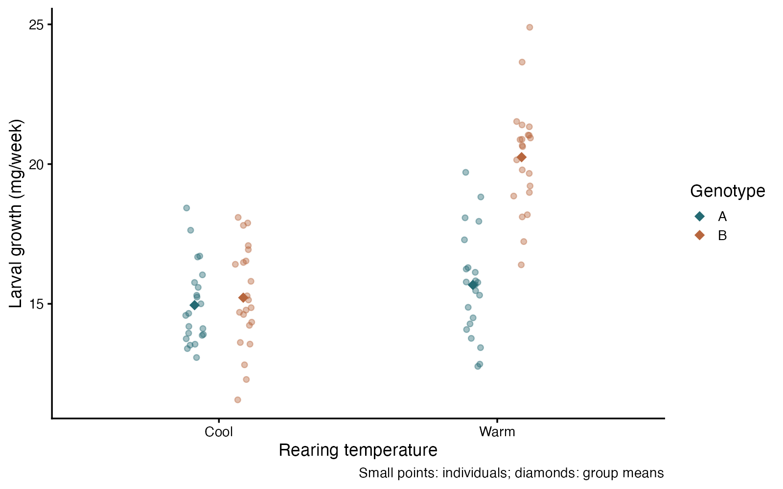
- Interaction = 4.30 mg/week
- 95% CI 2.80 to 5.81
- t(84) = 5.69; p = 1.78e-07
The warm-minus-cool growth effect was 4.30 mg/week greater in genotype B than A (95% CI 2.80 to 5.81; p = 1.78e-07). The interaction asks whether the temperature effect depends on genotype; a single average temperature effect would hide this difference.
**Teaching point:** An interaction is a difference of differences: a main-effect summary can conceal it.
### Analysis code excerpt
```r
d <- read.csv("modules/factorial_anova/generated/data.csv")
fit <- lm(growth ~ genotype * heat, data = d)
summary(fit)
interaction_ci <- confint(fit)["genotypeB:heatWarm", ]
```
The full script supplies package loading and any additional preparation.
### Full printed R output
```text
Call:
lm(formula = growth ~ genotype * heat, data = d)
Residuals:
Min 1Q Median 3Q Max
-3.8521 -1.1843 -0.0363 1.0850 4.6476
Coefficients:
Estimate Std. Error t value Pr(>|t|)
(Intercept) 14.9526 0.3779 39.567 < 2e-16 ***
genotypeB 0.2676 0.5344 0.501 0.618
heatWarm 0.7240 0.5344 1.355 0.179
genotypeB:heatWarm 4.3035 0.7558 5.694 1.78e-07 ***
---
Signif. codes: 0 ‘***’ 0.001 ‘**’ 0.01 ‘*’ 0.05 ‘.’ 0.1 ‘ ’ 1
Residual standard error: 1.773 on 84 degrees of freedom
Multiple R-squared: 0.6099, Adjusted R-squared: 0.5959
F-statistic: 43.77 on 3 and 84 DF, p-value: < 2.2e-16
```
### Recreate the observations
```r
output_dir <- "modules/factorial_anova/generated"
dir.create(output_dir, recursive = TRUE, showWarnings = FALSE)
set.seed(2101)
d <- expand.grid(replicate = 1:22, genotype = c("A", "B"),
heat = c("Cool", "Warm"))
d$growth <- with(d, 14 + 1.4 * (genotype == "B") +
2 * (heat == "Warm") + 2.3 * (genotype == "B" & heat == "Warm") +
rnorm(nrow(d), 0, 2.1))
write.csv(d, file.path(output_dir, "data.csv"), row.names = FALSE)
```
Run the complete module from the course folder:
```sh
Rscript modules/factorial_anova/analysis.R modules/factorial_anova/generated
```
## Dataset 15: ANCOVA: an adjusted group comparison
Plant ecologists compare nutrient treatment while accounting for initial plant height.
**Family:** ANOVA and contrasts · **Rows:** 90 · **Seed:** 2102
[Saved CSV](modules/ancova/generated/data.csv) · [Full runnable R script](modules/ancova/analysis.R) · [Full-size plot](modules/ancova/generated/plot.png)
**Generating truth:** The nutrient treatment increases the population mean biomass by 2.4 g at any shared initial height. Both groups have slope 1.5 g/cm. The adjusted treatment null is false.
**Exact generating model:** 45 independent plants are assigned to each treatment. Initial height is Uniform(3, 9) cm. Biomass = 2 + 1.5 × initial height + 2.4 if nutrient-treated + independent Normal(0, 1.8²) error, in g. No rounding is applied.
**Scientific question:** Do treatments differ in mean biomass at the same initial height?
**Null being tested / estimation target:** The treatment mean difference is zero at a common initial height in the stated model.
**Design and independent unit:** 90 independent plants; treatment groups overlap in initial height.
### Columns
| Column | Meaning | Unit / type |
|---|---|---|
| plant | Independent plant identifier | ID |
| treatment | Control or nutrient addition | category |
| initial | Height before treatment | cm |
| biomass | Final dry biomass | g |
### Analysis from the saved dataset
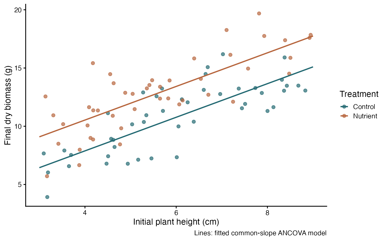
- Adjusted nutrient minus control = 2.65 g
- 95% CI 1.84 to 3.45
- t(87) = 6.55; p = 3.797e-09
At the same initial height, nutrient-treated plants had 2.65 g greater mean biomass (95% CI 1.84 to 3.45; p = 3.797e-09). This fitted model assumes a common height slope; the adjusted treatment comparison is supported by overlapping height ranges.
**Teaching point:** The scientific comparison holds the covariate fixed; the raw mean comparison is different.
### Analysis code excerpt
```r
d <- read.csv("modules/ancova/generated/data.csv")
fit <- lm(biomass ~ treatment + initial, data = d)
summary(fit)
adjusted_ci <- confint(fit)["treatmentNutrient", ]
```
The full script supplies package loading and any additional preparation.
### Full printed R output
```text
Call:
lm(formula = biomass ~ treatment + initial, data = d)
Residuals:
Min 1Q Median 3Q Max
-3.692 -1.195 0.030 1.050 4.634
Coefficients:
Estimate Std. Error t value Pr(>|t|)
(Intercept) 2.1147 0.7830 2.701 0.00831 **
treatmentNutrient 2.6479 0.4040 6.555 3.8e-09 ***
initial 1.4427 0.1212 11.900 < 2e-16 ***
---
Signif. codes: 0 ‘***’ 0.001 ‘**’ 0.01 ‘*’ 0.05 ‘.’ 0.1 ‘ ’ 1
Residual standard error: 1.899 on 87 degrees of freedom
Multiple R-squared: 0.6571, Adjusted R-squared: 0.6492
F-statistic: 83.35 on 2 and 87 DF, p-value: < 2.2e-16
```
### Recreate the observations
```r
output_dir <- "modules/ancova/generated"
dir.create(output_dir, recursive = TRUE, showWarnings = FALSE)
set.seed(2102)
d <- data.frame(plant = 1:90, treatment = rep(c("Control", "Nutrient"), each = 45),
initial = runif(90, 3, 9))
d$biomass <- with(d, 2 + 1.5 * initial +
2.4 * (treatment == "Nutrient") + rnorm(90, 0, 1.8))
write.csv(d, file.path(output_dir, "data.csv"), row.names = FALSE)
```
Run the complete module from the course folder:
```sh
Rscript modules/ancova/analysis.R modules/ancova/generated
```
## Dataset 16: Repeated-measures ANOVA
Physiologists measure the same animals at four assay temperatures.
**Family:** Repeated and clustered data · **Rows:** 96 · **Seed:** 2103
[Saved CSV](modules/repeated_anova/generated/data.csv) · [Full runnable R script](modules/repeated_anova/analysis.R) · [Full-size plot](modules/repeated_anova/generated/plot.png)
**Generating truth:** Population means are 8, 9.75, 11.5 and 13.25 µmol/hour. The endpoint difference is 5.25 µmol/hour and the equal-means null is false.
**Exact generating model:** 24 animals are measured at 15, 20, 25 and 30°C. Oxygen use = 8 + 0.35 × (temperature − 15) + an animal-specific Normal(0, 2²) intercept + independent Normal(0, 1.3²) observation error. Intercepts are shared within animals, producing repeated-measure dependence and a spherical covariance structure. No rounding is applied.
**Scientific question:** Are mean oxygen-use rates equal across temperatures within animals?
**Null being tested / estimation target:** All four population temperature means are equal.
**Design and independent unit:** Each of 24 animals provides all four measurements.
### Columns
| Column | Meaning | Unit / type |
|---|---|---|
| temperature | Assay temperature | °C |
| subject | Animal measured at all four temperatures | ID |
| oxygen | Measured oxygen consumption | µmol/hour |
### Analysis from the saved dataset
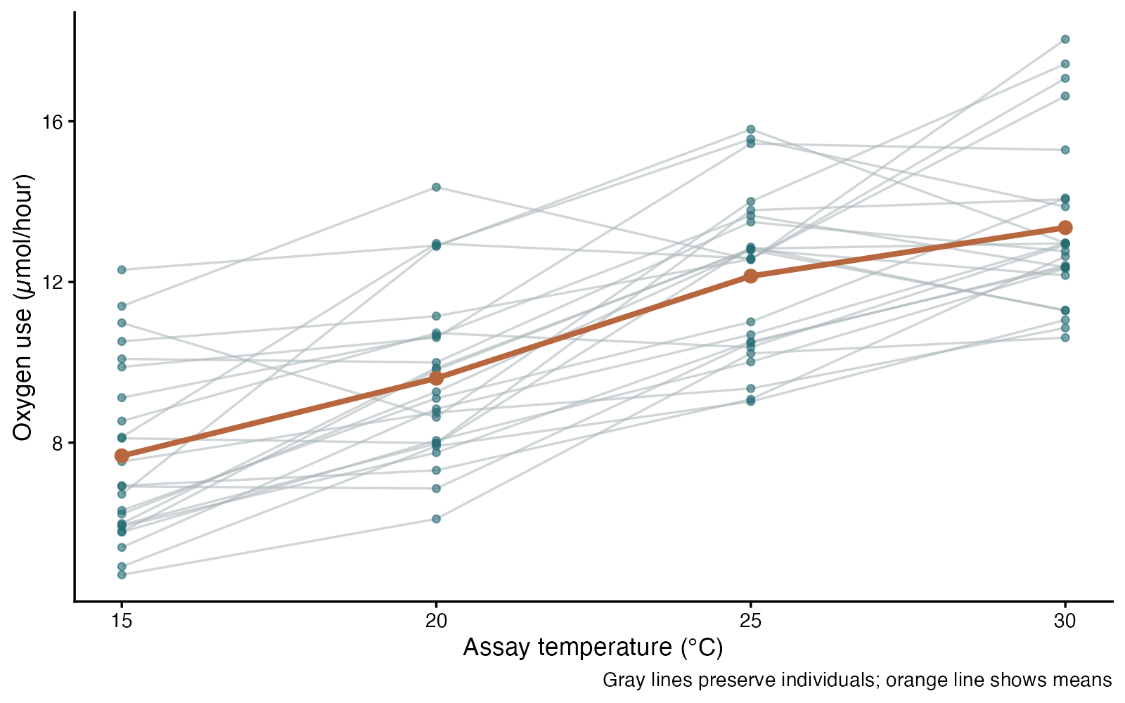
- Condition F(3, 69) = 84.32
- Omnibus p = 4.966e-23
- Planned 30−15°C mean difference = 5.68 µmol/hour
- 95% CI 4.99 to 6.38
Within the same 24 animals, temperature means differed (F(3, 69) = 84.32, p = 4.966e-23). The prespecified 30−15°C mean increase was 5.68 µmol/hour (95% CI 4.99 to 6.38). The repeated-measures F test assumes sphericity; the experiment has 24 independent animals, not 96 independent rows.
**Teaching point:** The subject ID, not the row, defines independent replication.
### Analysis code excerpt
```r
d <- read.csv("modules/repeated_anova/generated/data.csv")
fit <- aov(oxygen ~ condition + Error(subject/condition), data = d)
summary(fit)
endpoints <- t.test(d$oxygen[d$temperature == 30],
d$oxygen[d$temperature == 15], paired = TRUE)
```
The full script supplies package loading and any additional preparation.
### Full printed R output
```text
Error: subject
Df Sum Sq Mean Sq F value Pr(>F)
Residuals 23 285.9 12.43
Error: subject:condition
Df Sum Sq Mean Sq F value Pr(>F)
condition 3 467.9 155.98 84.32 <2e-16 ***
Residuals 69 127.6 1.85
---
Signif. codes: 0 ‘***’ 0.001 ‘**’ 0.01 ‘*’ 0.05 ‘.’ 0.1 ‘ ’ 1
```
### Recreate the observations
```r
output_dir <- "modules/repeated_anova/generated"
dir.create(output_dir, recursive = TRUE, showWarnings = FALSE)
set.seed(2103)
d <- expand.grid(temperature = c(15, 20, 25, 30), subject = 1:24)
individual <- rnorm(24, 0, 2)
d$oxygen <- 8 + .35 * (d$temperature - 15) +
individual[d$subject] + rnorm(nrow(d), 0, 1.3)
write.csv(d, file.path(output_dir, "data.csv"), row.names = FALSE)
```
Run the complete module from the course folder:
```sh
Rscript modules/repeated_anova/analysis.R modules/repeated_anova/generated
```
## Dataset 17: Friedman test
Sensory biologists record activity scores from each insect under three light conditions.
**Family:** Nonparametric alternatives · **Rows:** 54 · **Seed:** 1108
[Saved CSV](modules/friedman/generated/data.csv) · [Full runnable R script](modules/friedman/analysis.R) · [Full-size plot](modules/friedman/generated/plot.png)
**Generating truth:** Condition effects exist before rounding (0, +0.8, +1.6), and condition score distributions differ after rounding. Repeated observations share an insect baseline.
**Exact generating model:** 18 insects each receive all 3 conditions. Each insect has a Normal(5, 1.3 SD) baseline; Dim, Moderate, and Bright add 0, 0.8, and 1.6. Independent Normal(0, 1 SD) noise is added, then scores are rounded and restricted to 0–10.
**Scientific question:** Do light conditions differ after accounting for insect-to-insect variation?
**Null being tested / estimation target:** Within blocks, condition labels are exchangeable: no systematic condition effect.
**Design and independent unit:** Eighteen independent insects each complete all three conditions in randomized order.
### Columns
| Column | Meaning | Unit / type |
|---|---|---|
| insect | Independent insect/block identifier | none |
| condition | Light condition | category |
| activity_score | Rounded and bounded activity measure | score 0 to 10 |
### Analysis from the saved dataset
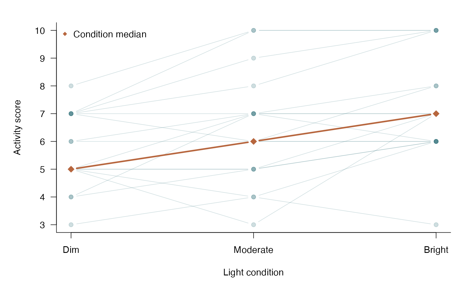
- Independent blocks = 18; conditions = 3
- Friedman chi-square = 17.63; df = 2; p = 0.0001482
- Condition medians: Dim 5; Moderate 6; Bright 7
For 18 insects measured under all three conditions, the Friedman comparison gave chi-square(2) = 17.63, p = 0.0001482. This tests a systematic condition effect within insects; it does not identify which conditions differ.
**Teaching point:** Rank within each insect so that between-insect differences do not masquerade as condition effects.
### Analysis code excerpt
```r
d <- read.csv("modules/friedman/generated/data.csv")
d$condition <- factor(d$condition, levels = c("Dim", "Moderate", "Bright"))
d$insect <- factor(d$insect)
fit <- friedman.test(activity_score ~ condition | insect, data = d)
```
The full script supplies package loading and any additional preparation.
### Full printed R output
```text
Friedman rank sum test
data: activity_score and condition and insect
Friedman chi-squared = 17.633, df = 2, p-value = 0.0001482
```
### Recreate the observations
```r
output_dir <- "modules/friedman/generated"
dir.create(output_dir, recursive = TRUE, showWarnings = FALSE)
set.seed(1108)
insect <- rep(1:18, each = 3)
condition <- rep(c("Dim", "Moderate", "Bright"), 18)
score <- pmax(0, pmin(10, round(rep(rnorm(18, 5, 1.3), each = 3) +
rep(c(0, .8, 1.6), 18) + rnorm(54, 0, 1))))
d <- data.frame(insect, condition, activity_score = score)
write.csv(d, file.path(output_dir, "data.csv"), row.names = FALSE)
```
Run the complete module from the course folder:
```sh
Rscript modules/friedman/analysis.R modules/friedman/generated
```
## Dataset 18: Tukey / Tukey–Kramer comparisons
Plant growth is compared across four nutrient regimes.
**Family:** ANOVA and contrasts · **Rows:** 80 · **Seed:** 2104
[Saved CSV](modules/tukey/generated/data.csv) · [Full runnable R script](modules/tukey/analysis.R) · [Full-size plot](modules/tukey/generated/plot.png)
**Generating truth:** Population means for A–D are 8, 9, 11.3 and 12.1 g; all distinct pairwise mean-equality nulls are false.
**Exact generating model:** 20 independent plants per nutrient regime have normal biomass with means 8, 9, 11.3 and 12.1 g for A–D and a common SD of 1.7 g. Values are not rounded. The identical dataset is regenerated separately for each comparison procedure.
**Scientific question:** Which pairs of nutrient means differ?
**Null being tested / estimation target:** For each pair, the two population means are equal.
**Design and independent unit:** 20 independent plants per regime; all procedures use the same simulated dataset.
### Columns
| Column | Meaning | Unit / type |
|---|---|---|
| plant | Independent plant identifier | ID |
| nutrient | Nutrient regime A–D | category |
| biomass | Dry biomass | g |
### Analysis from the saved dataset
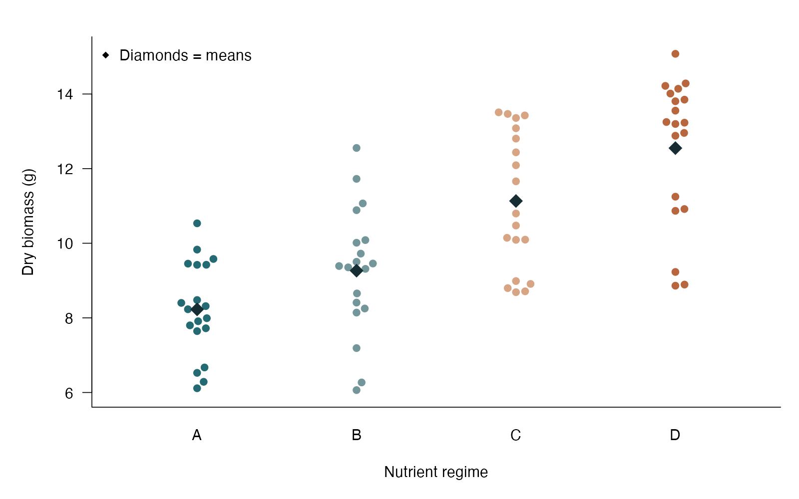
- Family: all six pairwise nutrient comparisons
- D minus C = 1.42 g
- Simultaneous 95% CI 0.04 to 2.80
- Tukey-adjusted p = 0.0415
Regime D exceeded C by 1.42 g (simultaneous 95% CI 0.04 to 2.80; Tukey-adjusted p = 0.0415). The interval and p-value account for all six pairwise comparisons; they do not protect every possible weighted contrast.
**Teaching point:** Protect the family of all six pairwise mean comparisons.
### Analysis code excerpt
```r
d <- read.csv("modules/tukey/generated/data.csv")
fit <- aov(biomass ~ nutrient, data = d)
comparisons <- TukeyHSD(fit, "nutrient", conf.level = .95)
comparisons
```
The full script supplies package loading and any additional preparation.
### Full printed R output
```text
Df Sum Sq Mean Sq F value Pr(>F)
nutrient 3 222.4 74.14 26.94 5.68e-12 ***
Residuals 76 209.2 2.75
---
Signif. codes: 0 ‘***’ 0.001 ‘**’ 0.01 ‘*’ 0.05 ‘.’ 0.1 ‘ ’ 1
Tukey multiple comparisons of means
95% family-wise confidence level
Fit: aov(formula = biomass ~ nutrient, data = d)
$nutrient
diff lwr upr p adj
B-A 1.037343 -0.34073261 2.415418 0.2056314
C-A 2.905036 1.52696022 4.283111 0.0000025
D-A 4.322102 2.94402599 5.700177 0.0000000
C-B 1.867693 0.48961729 3.245768 0.0035291
D-B 3.284759 1.90668306 4.662834 0.0000001
D-C 1.417066 0.03899023 2.795141 0.0415003
```
### Recreate the observations
```r
output_dir <- "modules/tukey/generated"
dir.create(output_dir, recursive = TRUE, showWarnings = FALSE)
set.seed(2104)
d <- data.frame(plant = 1:80,
nutrient = rep(c("A", "B", "C", "D"), each = 20))
d$biomass <- rnorm(80, rep(c(8, 9, 11.3, 12.1), each = 20), 1.7)
write.csv(d, file.path(output_dir, "data.csv"), row.names = FALSE)
```
Run the complete module from the course folder:
```sh
Rscript modules/tukey/analysis.R modules/tukey/generated
```
## Dataset 19: Fisher least significant difference
Plant growth is compared across four nutrient regimes.
**Family:** ANOVA and contrasts · **Rows:** 80 · **Seed:** 2104
[Saved CSV](modules/fisher_lsd/generated/data.csv) · [Full runnable R script](modules/fisher_lsd/analysis.R) · [Full-size plot](modules/fisher_lsd/generated/plot.png)
**Generating truth:** Population means for A–D are 8, 9, 11.3 and 12.1 g; all distinct pairwise mean-equality nulls are false.
**Exact generating model:** 20 independent plants per nutrient regime have normal biomass with means 8, 9, 11.3 and 12.1 g for A–D and a common SD of 1.7 g. Values are not rounded. The identical dataset is regenerated separately for each comparison procedure.
**Scientific question:** What does an unadjusted pairwise comparison after the ANOVA gate test?
**Null being tested / estimation target:** For a chosen pair, the two population means are equal.
**Design and independent unit:** 20 independent plants per regime; all procedures use the same simulated dataset.
### Columns
| Column | Meaning | Unit / type |
|---|---|---|
| plant | Independent plant identifier | ID |
| nutrient | Nutrient regime A–D | category |
| biomass | Dry biomass | g |
### Analysis from the saved dataset
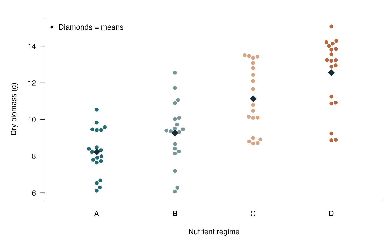
- Omnibus p = 5.683e-12
- A - B = -1.04 g
- Individual 95% CI -2.08 to 0.01
- Unadjusted p = 0.05163
- Protected LSD first requires a significant omnibus test.
The omnibus test had p = 5.683e-12, so the protected LSD gate is passed in this example. The A - B difference was -1.04 g (individual 95% CI -2.08 to 0.01; unadjusted p = 0.05163). This gate does not generally protect all pairwise decisions when some of four or more means differ; use Tukey for the all-pairs family.
**Teaching point:** An omnibus gate plus unadjusted comparisons is not general all-pairs protection.
### Analysis code excerpt
```r
d <- read.csv("modules/fisher_lsd/generated/data.csv")
fit <- lm(biomass ~ nutrient, data = d)
omnibus_p <- anova(fit)$`Pr(>F)`[1]
means <- emmeans::emmeans(fit, ~ nutrient)
comparisons <- NULL
if (omnibus_p < .05) {
comparisons <- summary(emmeans::contrast(means, "pairwise"),
infer = c(TRUE, TRUE), adjust = "none")
}
```
The full script supplies package loading and any additional preparation.
### Full printed R output
```text
Call:
lm(formula = biomass ~ nutrient, data = d)
Residuals:
Min 1Q Median 3Q Max
-3.6874 -1.0377 0.1064 1.2669 3.2888
Coefficients:
Estimate Std. Error t value Pr(>|t|)
(Intercept) 8.2277 0.3710 22.179 < 2e-16 ***
nutrientB 1.0373 0.5246 1.977 0.0516 .
nutrientC 2.9050 0.5246 5.537 4.21e-07 ***
nutrientD 4.3221 0.5246 8.239 3.85e-12 ***
---
Signif. codes: 0 ‘***’ 0.001 ‘**’ 0.01 ‘*’ 0.05 ‘.’ 0.1 ‘ ’ 1
Residual standard error: 1.659 on 76 degrees of freedom
Multiple R-squared: 0.5153, Adjusted R-squared: 0.4962
F-statistic: 26.94 on 3 and 76 DF, p-value: 5.683e-12
contrast estimate SE df lower.CL upper.CL t.ratio p.value
A - B -1.04 0.525 76 -2.08 0.00753 -1.977 0.0516
A - C -2.91 0.525 76 -3.95 -1.86016 -5.537 <0.0001
A - D -4.32 0.525 76 -5.37 -3.27723 -8.239 <0.0001
B - C -1.87 0.525 76 -2.91 -0.82282 -3.560 0.0006
B - D -3.28 0.525 76 -4.33 -2.23988 -6.261 <0.0001
C - D -1.42 0.525 76 -2.46 -0.37219 -2.701 0.0085
Confidence level used: 0.95
```
### Recreate the observations
```r
output_dir <- "modules/fisher_lsd/generated"
dir.create(output_dir, recursive = TRUE, showWarnings = FALSE)
set.seed(2104)
d <- data.frame(plant = 1:80,
nutrient = rep(c("A", "B", "C", "D"), each = 20))
d$biomass <- rnorm(80, rep(c(8, 9, 11.3, 12.1), each = 20), 1.7)
write.csv(d, file.path(output_dir, "data.csv"), row.names = FALSE)
```
Run the complete module from the course folder:
```sh
Rscript modules/fisher_lsd/analysis.R modules/fisher_lsd/generated
```
## Dataset 20: Scheffé contrasts
Plant growth is compared across four nutrient regimes.
**Family:** ANOVA and contrasts · **Rows:** 80 · **Seed:** 2104
[Saved CSV](modules/scheffe/generated/data.csv) · [Full runnable R script](modules/scheffe/analysis.R) · [Full-size plot](modules/scheffe/generated/plot.png)
**Generating truth:** Population means for A–D are 8, 9, 11.3 and 12.1 g; all distinct pairwise mean-equality nulls are false. The specified (C+D)/2 − (A+B)/2 contrast equals 3.2 g.
**Exact generating model:** 20 independent plants per nutrient regime have normal biomass with means 8, 9, 11.3 and 12.1 g for A–D and a common SD of 1.7 g. Values are not rounded. The identical dataset is regenerated separately for each comparison procedure.
**Scientific question:** Does the average of regimes C and D differ from the average of A and B?
**Null being tested / estimation target:** The contrast (μC + μD)/2 − (μA + μB)/2 is zero.
**Design and independent unit:** 20 independent plants per regime; all procedures use the same simulated dataset.
### Columns
| Column | Meaning | Unit / type |
|---|---|---|
| plant | Independent plant identifier | ID |
| nutrient | Nutrient regime A–D | category |
| biomass | Dry biomass | g |
### Analysis from the saved dataset
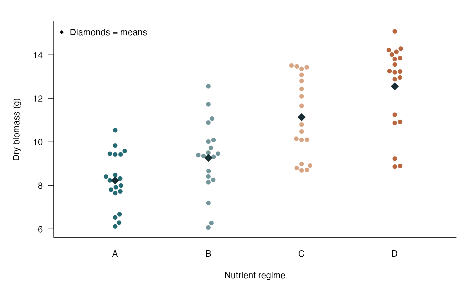
- Contrast: (C + D)/2 − (A + B)/2
- Estimated difference = 3.09 g
- Scheffé 95% CI 2.03 to 4.16
- Scheffé-adjusted p = 9.177e-11
The average of regimes C and D exceeded the average of A and B by 3.09 g (Scheffé simultaneous 95% CI 2.03 to 4.16; adjusted p = 9.177e-11). Using rank 3 protects all mean contrasts among these four groups, a larger family than the pairwise comparisons protected by Tukey.
**Teaching point:** A weighted contrast asks a specific biological question; Scheffé protects the larger all-contrast family.
### Analysis code excerpt
```r
d <- read.csv("modules/scheffe/generated/data.csv")
fit <- lm(biomass ~ nutrient, data = d)
means <- emmeans::emmeans(fit, ~ nutrient)
contrast <- emmeans::contrast(means,
list("CD average minus AB average" = c(-.5, -.5, .5, .5)))
comparison <- summary(contrast, infer = c(TRUE, TRUE),
adjust = "scheffe", scheffe.rank = 3)
```
The full script supplies package loading and any additional preparation.
### Full printed R output
```text
Call:
lm(formula = biomass ~ nutrient, data = d)
Residuals:
Min 1Q Median 3Q Max
-3.6874 -1.0377 0.1064 1.2669 3.2888
Coefficients:
Estimate Std. Error t value Pr(>|t|)
(Intercept) 8.2277 0.3710 22.179 < 2e-16 ***
nutrientB 1.0373 0.5246 1.977 0.0516 .
nutrientC 2.9050 0.5246 5.537 4.21e-07 ***
nutrientD 4.3221 0.5246 8.239 3.85e-12 ***
---
Signif. codes: 0 ‘***’ 0.001 ‘**’ 0.01 ‘*’ 0.05 ‘.’ 0.1 ‘ ’ 1
Residual standard error: 1.659 on 76 degrees of freedom
Multiple R-squared: 0.5153, Adjusted R-squared: 0.4962
F-statistic: 26.94 on 3 and 76 DF, p-value: 5.683e-12
contrast estimate SE df lower.CL upper.CL t.ratio
CD average minus AB average 3.09 0.371 76 2.03 4.16 8.343
p.value
<0.0001
Confidence level used: 0.95
Conf-level adjustment: scheffe method with rank 3
P value adjustment: scheffe method with rank 3
```
### Recreate the observations
```r
output_dir <- "modules/scheffe/generated"
dir.create(output_dir, recursive = TRUE, showWarnings = FALSE)
set.seed(2104)
d <- data.frame(plant = 1:80,
nutrient = rep(c("A", "B", "C", "D"), each = 20))
d$biomass <- rnorm(80, rep(c(8, 9, 11.3, 12.1), each = 20), 1.7)
write.csv(d, file.path(output_dir, "data.csv"), row.names = FALSE)
```
Run the complete module from the course folder:
```sh
Rscript modules/scheffe/analysis.R modules/scheffe/generated
```
## Dataset 21: Dunn rank comparisons
Ecologists compare skewed leaf-damage measurements among four treatments.
**Family:** Rank methods · **Rows:** 84 · **Seed:** 2105
[Saved CSV](modules/dunn/generated/data.csv) · [Full runnable R script](modules/dunn/analysis.R) · [Full-size plot](modules/dunn/generated/plot.png)
**Generating truth:** Group distributions differ; their population medians are exp(1.2), exp(1.3), exp(1.7) and exp(1.9) mm². Dunn tests pooled-rank tendencies, not arithmetic mean equality. The distributions also differ in original-scale spread.
**Exact generating model:** 21 independent leaves in each of four groups have log-normal damage. Log damage is Normal(mean, 0.48²), with means 1.2, 1.3, 1.7 and 1.9 for A–D. Damage remains positive and unrounded. All leaves come from different plants.
**Scientific question:** Which pairs differ in their rank tendencies?
**Null being tested / estimation target:** For a chosen pair, pooled-rank tendencies are equal under the common-distribution null.
**Design and independent unit:** 21 independent leaves from different plants per treatment.
### Columns
| Column | Meaning | Unit / type |
|---|---|---|
| leaf | Independent leaf from a distinct plant | ID |
| treatment | Treatment A–D | category |
| damage | Area removed from a leaf | mm² |
### Analysis from the saved dataset
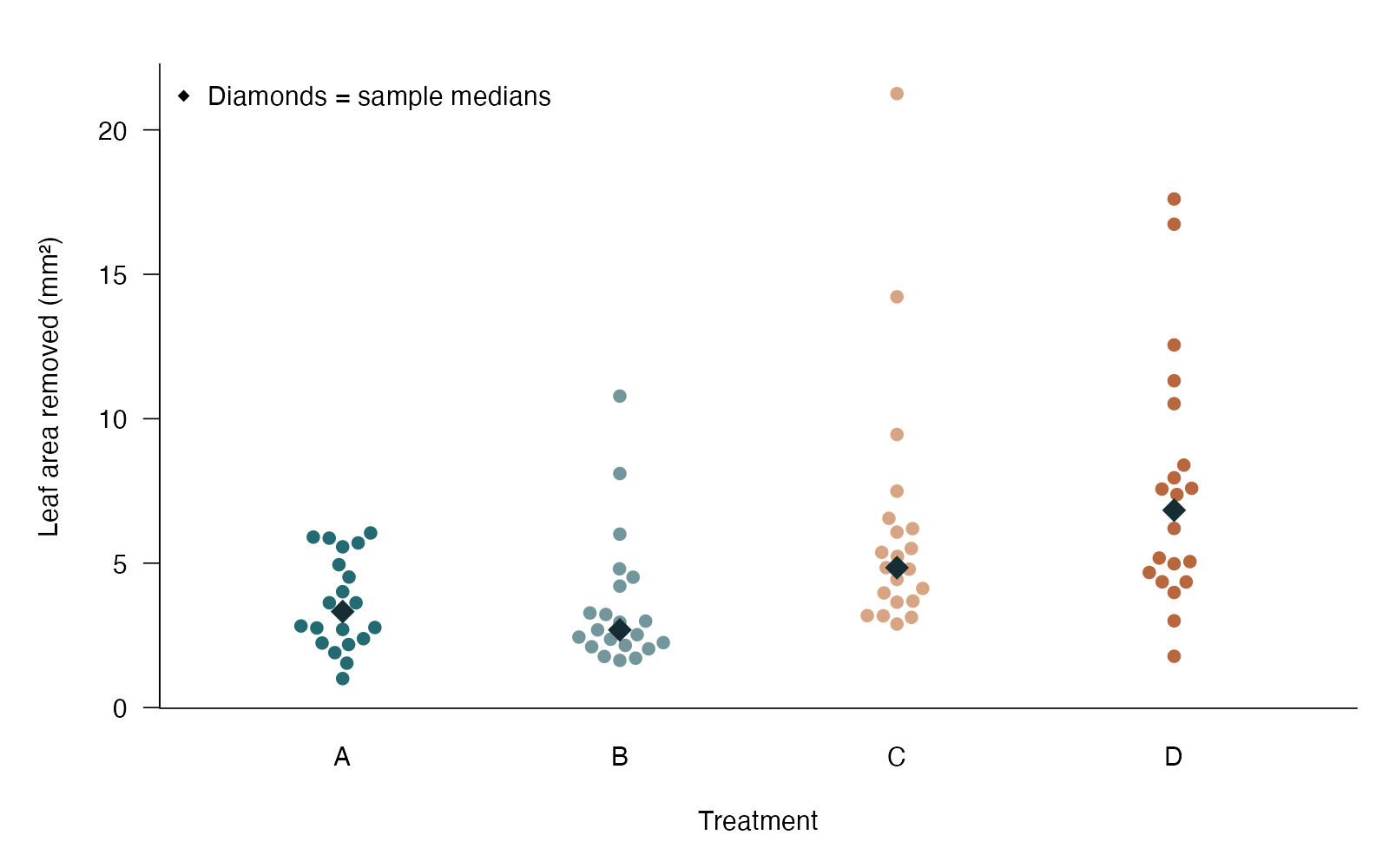
- Kruskal–Wallis p = 1.352e-05
- Highlighted pair: B - D
- Dunn z = -4.30
- Two-sided Holm-adjusted p = 0.0001018
Across the six rank comparisons, the highlighted B - D comparison had Dunn z = -4.30 and two-sided Holm-adjusted p = 0.0001018. This compares pooled rank tendencies; with unequal distribution shapes, it is not simply a test of equal medians. The smallest adjusted p-value is highlighted after protecting the full six-pair family.
**Teaching point:** After choosing a rank question, retain multiplicity protection for pairwise follow-ups.
### Analysis code excerpt
```r
d <- read.csv("modules/dunn/generated/data.csv")
overall <- kruskal.test(damage ~ treatment, data = d)
comparisons <- dunn.test::dunn.test(d$damage, d$treatment,
method = "holm", altp = TRUE, kw = FALSE, list = FALSE)
```
The full script supplies package loading and any additional preparation.
### Full printed R output
```text
Kruskal-Wallis rank sum test
data: damage by treatment
Kruskal-Wallis chi-squared = 25.276, df = 3, p-value = 1.352e-05
$chi2
[1] 25.27627
$Z
[1] 0.5693239 -2.5682832 -3.1376070 -3.7322342 -4.3015580 -1.1639510
$altP
[1] 5.691364e-01 1.022036e-02 1.703331e-03 1.897889e-04 1.696014e-05
[6] 2.444439e-01
$altP.adjusted
[1] 0.5691363809 0.0306610890 0.0068133231 0.0009489447 0.0001017608
[6] 0.4888877458
$comparisons
[1] "A - B" "A - C" "B - C" "A - D" "B - D" "C - D"
```
### Recreate the observations
```r
output_dir <- "modules/dunn/generated"
dir.create(output_dir, recursive = TRUE, showWarnings = FALSE)
set.seed(2105)
d <- data.frame(leaf = 1:84,
treatment = rep(c("A", "B", "C", "D"), each = 21))
d$damage <- rlnorm(84, rep(c(1.2, 1.3, 1.7, 1.9), each = 21), .48)
write.csv(d, file.path(output_dir, "data.csv"), row.names = FALSE)
```
Run the complete module from the course folder:
```sh
Rscript modules/dunn/analysis.R modules/dunn/generated
```
## Dataset 22: Pearson correlation
Evolutionary biologists measure wing and tail lengths in adult birds from a single population.
**Family:** Association · **Rows:** 45 · **Seed:** 1112
[Saved CSV](modules/pearson/generated/data.csv) · [Full runnable R script](modules/pearson/analysis.R) · [Full-size plot](modules/pearson/generated/plot.png)
**Generating truth:** The generating population Pearson correlation is 0.55*5 / sqrt((0.55*5)^2 + 3.5^2), approximately 0.618. It is not the observed sample correlation.
**Exact generating model:** 45 independent wing lengths are Normal(75, 5 SD). Tail length is 15 + 0.55 times wing length + independent Normal(0, 3.5 SD) noise.
**Scientific question:** Are wing and tail lengths linearly associated in this population?
**Null being tested / estimation target:** The population Pearson correlation is zero.
**Design and independent unit:** Each independent bird contributes one pair of continuous traits.
### Columns
| Column | Meaning | Unit / type |
|---|---|---|
| bird | Independent bird identifier | none |
| wing_mm | Wing length | mm |
| tail_mm | Tail length | mm |
### Analysis from the saved dataset
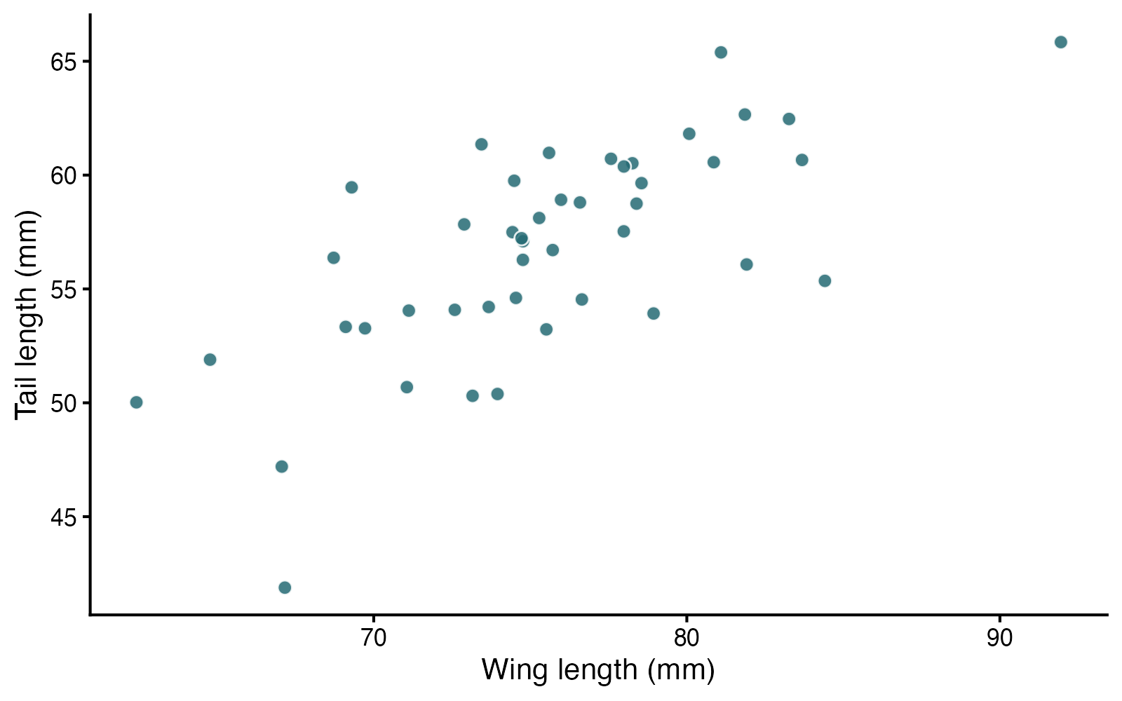
- Pearson r = 0.700
- 95% CI for population correlation: 0.512 to 0.824
- t = 6.43; df = 43; p = 8.606e-08
Wing and tail lengths had Pearson r = 0.700 (95% CI 0.512 to 0.824), p = 8.606e-08. This describes linear association within the sampled population; it does not establish that one trait causes the other.
**Teaching point:** Correlation describes linear association symmetrically; causal direction and a slope are separate questions.
### Analysis code excerpt
```r
d <- read.csv("modules/pearson/generated/data.csv")
fit <- cor.test(d$wing_mm, d$tail_mm, method = "pearson",
alternative = "two.sided", conf.level = .95)
```
The full script supplies package loading and any additional preparation.
### Full printed R output
```text
Pearson's product-moment correlation
data: d$wing_mm and d$tail_mm
t = 6.4317, df = 43, p-value = 8.606e-08
alternative hypothesis: true correlation is not equal to 0
95 percent confidence interval:
0.5119136 0.8243291
sample estimates:
cor
0.7002284
```
### Recreate the observations
```r
output_dir <- "modules/pearson/generated"
dir.create(output_dir, recursive = TRUE, showWarnings = FALSE)
set.seed(1112)
wing <- rnorm(45, 75, 5)
tail <- 15 + .55 * wing + rnorm(45, 0, 3.5)
d <- data.frame(bird = 1:45, wing_mm = wing, tail_mm = tail)
write.csv(d, file.path(output_dir, "data.csv"), row.names = FALSE)
```
Run the complete module from the course folder:
```sh
Rscript modules/pearson/analysis.R modules/pearson/generated
```
## Dataset 23: Spearman rank correlation
Microbial ecologists compare soil salinity with bacterial richness across independent soil cores.
**Family:** Nonparametric alternatives · **Rows:** 45 · **Seed:** 1113
[Saved CSV](modules/spearman/generated/data.csv) · [Full runnable R script](modules/spearman/analysis.R) · [Full-size plot](modules/spearman/generated/plot.png)
**Generating truth:** The underlying mean response decreases nonlinearly with salinity, creating a negative monotonic association. No fixed numeric population Spearman coefficient was specified.
**Exact generating model:** 45 independent site salinities are Uniform(0.5, 8). Richness is 90 - 25*log(salinity + 1) + Normal(0, 7 SD) noise, rounded to the nearest taxon.
**Scientific question:** Does bacterial richness tend to decline as salinity increases?
**Null being tested / estimation target:** The population Spearman rank correlation is zero.
**Design and independent unit:** Forty-five independent sites contribute one salinity and richness measurement each.
### Columns
| Column | Meaning | Unit / type |
|---|---|---|
| site | Independent site identifier | none |
| salinity_ppt | Soil salinity | parts per thousand |
| richness | Observed bacterial taxon richness | taxa |
### Analysis from the saved dataset
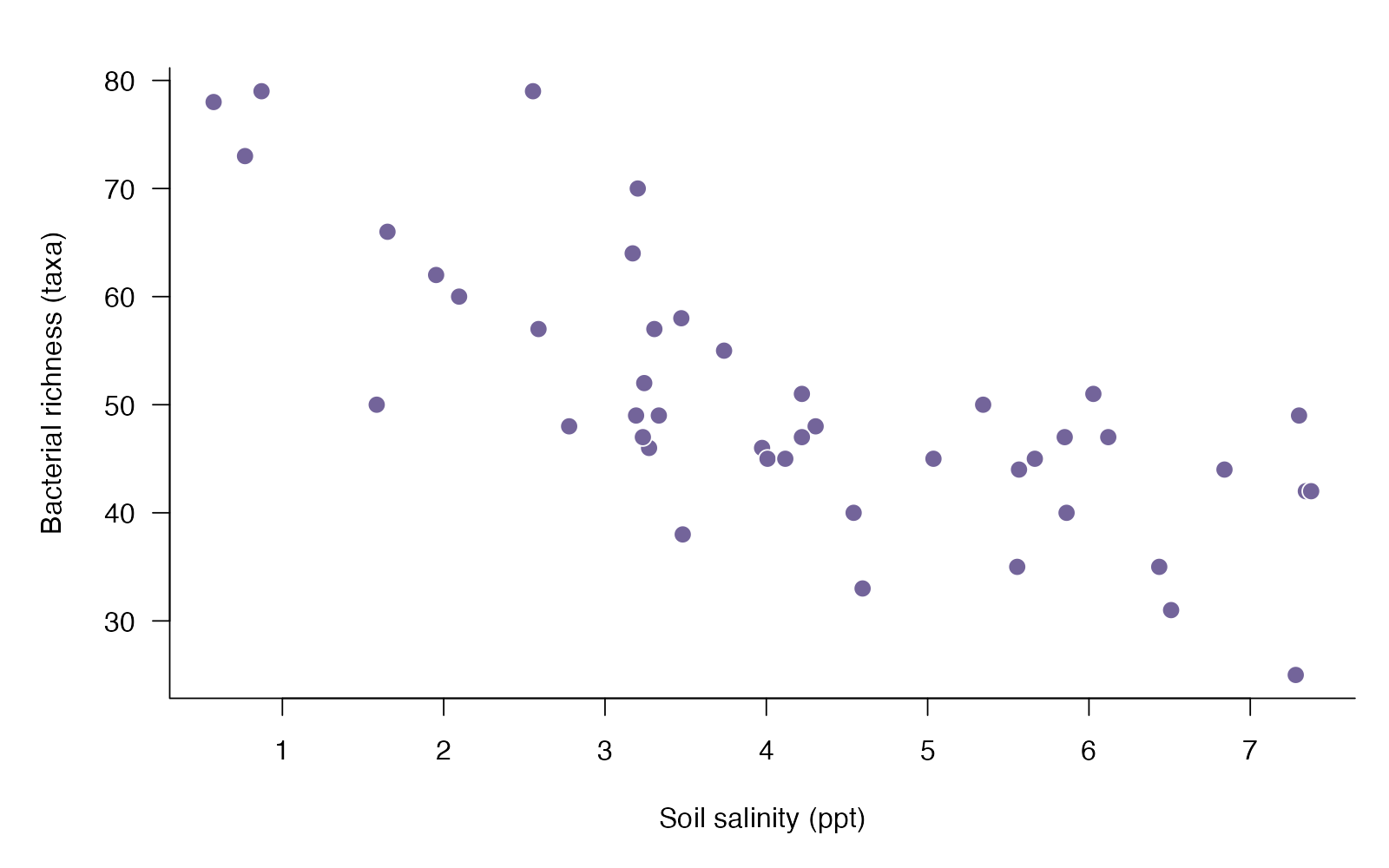
- Spearman rho = -0.752; n = 45
- S = 26599.8; asymptotic two-sided p = 2.549e-09
- The coefficient describes rank association, not a change in taxa per ppt.
Salinity and bacterial richness had Spearman rho = -0.752 (two-sided p = 2.549e-09). This quantifies their monotonic rank association. It does not estimate a change in mean richness per unit salinity.
**Teaching point:** Ranks can summarize a monotonic curve without claiming a constant change in the original response units.
### Analysis code excerpt
```r
d <- read.csv("modules/spearman/generated/data.csv")
fit <- cor.test(d$salinity_ppt, d$richness,
method = "spearman", exact = FALSE,
alternative = "two.sided")
```
The full script supplies package loading and any additional preparation.
### Full printed R output
```text
Spearman's rank correlation rho
data: d$salinity_ppt and d$richness
S = 26600, p-value = 2.549e-09
alternative hypothesis: true rho is not equal to 0
sample estimates:
rho
-0.7522922
```
### Recreate the observations
```r
output_dir <- "modules/spearman/generated"
dir.create(output_dir, recursive = TRUE, showWarnings = FALSE)
set.seed(1113)
salinity <- runif(45, .5, 8)
richness <- round(90 - 25 * log(salinity + 1) + rnorm(45, 0, 7))
d <- data.frame(site = 1:45, salinity_ppt = salinity, richness = richness)
write.csv(d, file.path(output_dir, "data.csv"), row.names = FALSE)
```
Run the complete module from the course folder:
```sh
Rscript modules/spearman/analysis.R modules/spearman/generated
```
## Dataset 24: Simple linear regression
Plant ecologists grow seedlings under a gradient of nitrogen supply.
**Family:** Regression · **Rows:** 36 · **Seed:** 1114
[Saved CSV](modules/simple_lm/generated/data.csv) · [Full runnable R script](modules/simple_lm/analysis.R) · [Full-size plot](modules/simple_lm/generated/plot.png)
**Generating truth:** The conditional mean intercept is 2.2 g and slope is +0.42 g per mg nitrogen. The zero-slope null is false.
**Exact generating model:** 36 nitrogen doses are Uniform(0, 12) mg. Independent biomass values follow 2.2 + 0.42*nitrogen + Normal(0, 0.8 SD).
**Scientific question:** How much does mean seedling biomass change per additional mg of nitrogen?
**Null being tested / estimation target:** The population slope of mean biomass on nitrogen is zero.
**Design and independent unit:** Thirty-six independently assigned pots receive one nitrogen level and yield one biomass measurement.
### Columns
| Column | Meaning | Unit / type |
|---|---|---|
| pot | Independent pot identifier | none |
| nitrogen_mg | Assigned nitrogen dose | mg |
| biomass_g | Seedling biomass | g |
### Analysis from the saved dataset
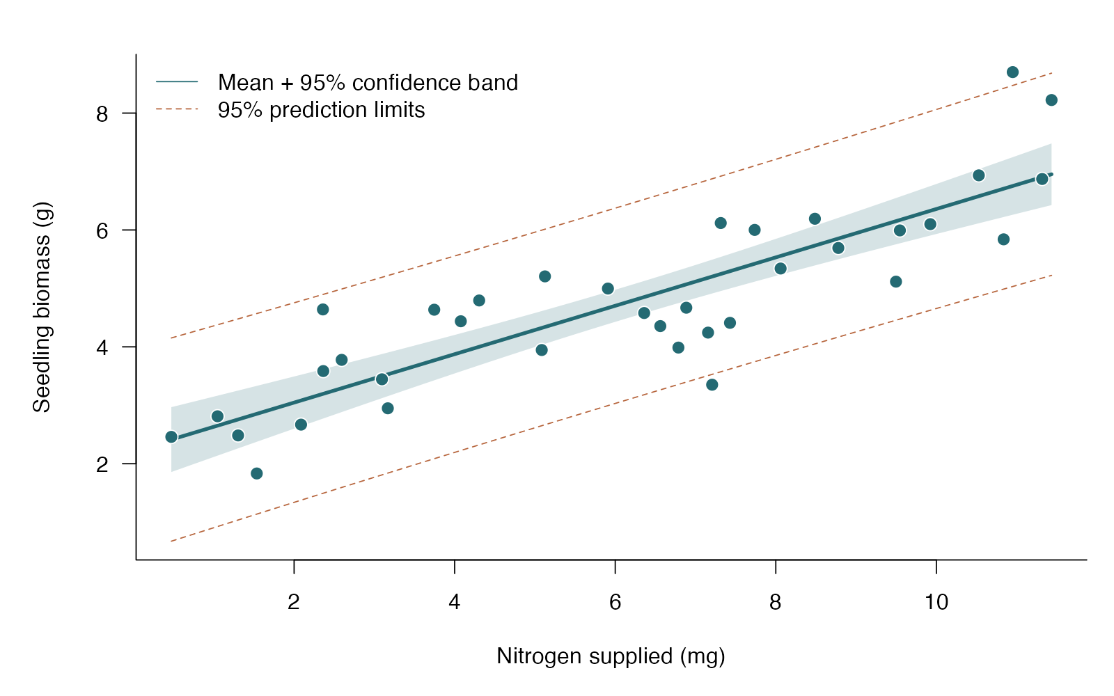
- Slope = 0.414 g biomass per mg nitrogen
- 95% slope CI: 0.329 to 0.499
- Slope t = 9.90; df = 34; p = 1.525e-11
- R-squared = 0.742
Each additional mg of nitrogen was associated with 0.414 g higher mean biomass (95% CI 0.329 to 0.499); slope t(34) = 9.90, p = 1.525e-11. The narrow band concerns mean biomass; the wider prediction limits concern a new individual pot.
**Teaching point:** Choose confidence intervals for a mean response and prediction intervals for a new individual pot.
### Analysis code excerpt
```r
d <- read.csv("modules/simple_lm/generated/data.csv")
fit <- lm(biomass_g ~ nitrogen_mg, data = d)
coefficients <- summary(fit)$coefficients
ci <- confint(fit)
grid <- data.frame(nitrogen_mg = seq(min(d$nitrogen_mg), max(d$nitrogen_mg), length.out = 100))
mean_ci <- predict(fit, grid, interval = "confidence")
new_pot <- predict(fit, grid, interval = "prediction")
```
The full script supplies package loading and any additional preparation.
### Full printed R output
```text
Call:
lm(formula = biomass_g ~ nitrogen_mg, data = d)
Residuals:
Min 1Q Median 3Q Max
-1.8507 -0.4546 -0.1079 0.4972 1.9486
Coefficients:
Estimate Std. Error t value Pr(>|t|)
(Intercept) 2.21791 0.29034 7.639 7.05e-09 ***
nitrogen_mg 0.41409 0.04185 9.896 1.52e-11 ***
---
Signif. codes: 0 ‘***’ 0.001 ‘**’ 0.01 ‘*’ 0.05 ‘.’ 0.1 ‘ ’ 1
Residual standard error: 0.811 on 34 degrees of freedom
Multiple R-squared: 0.7423, Adjusted R-squared: 0.7347
F-statistic: 97.93 on 1 and 34 DF, p-value: 1.525e-11
2.5 % 97.5 %
(Intercept) 1.6278685 2.8079514
nitrogen_mg 0.3290528 0.4991331
```
### Recreate the observations
```r
output_dir <- "modules/simple_lm/generated"
dir.create(output_dir, recursive = TRUE, showWarnings = FALSE)
set.seed(1114)
nitrogen <- runif(36, 0, 12)
biomass <- 2.2 + .42 * nitrogen + rnorm(36, 0, .8)
d <- data.frame(pot = 1:36, nitrogen_mg = nitrogen, biomass_g = biomass)
write.csv(d, file.path(output_dir, "data.csv"), row.names = FALSE)
```
Run the complete module from the course folder:
```sh
Rscript modules/simple_lm/analysis.R modules/simple_lm/generated
```
## Dataset 25: Multiple linear regression
Evolutionary biologists relate beetle horn length to body size and larval nutrition.
**Family:** Regression · **Rows:** 60 · **Seed:** 1115
[Saved CSV](modules/multiple_lm/generated/data.csv) · [Full runnable R script](modules/multiple_lm/analysis.R) · [Full-size plot](modules/multiple_lm/generated/plot.png)
**Generating truth:** The true conditional body slope is 0.35 mm/mm and nutrition slope 0.16 mm/mg, with no interaction. Both zero-coefficient nulls are false.
**Exact generating model:** 60 independent body lengths are Uniform(7, 12) mm and nutrition values independently Uniform(2, 10) mg. Horn length = 0.4 + 0.35*body + 0.16*nutrition + Normal(0, 0.65 SD).
**Scientific question:** Does body size predict mean horn length after accounting for larval nutrition?
**Null being tested / estimation target:** The body-size coefficient is zero conditional on nutrition in the specified model.
**Design and independent unit:** Sixty independent beetles are raised across a nutrient gradient and measured as adults.
### Columns
| Column | Meaning | Unit / type |
|---|---|---|
| beetle | Independent beetle identifier | none |
| body_mm | Adult body length | mm |
| nutrition_mg | Larval nutrition amount | mg |
| horn_mm | Adult horn length | mm |
### Analysis from the saved dataset
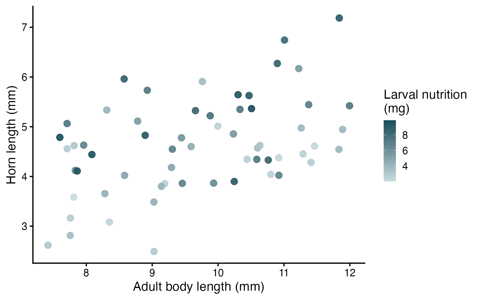
- Body slope, adjusted for nutrition = 0.299 mm/mm
- 95% CI: 0.159 to 0.440
- Body coefficient p = 7.658e-05; nested-model F = 18.17
- Nutrition slope = 0.181 mm/mg; p = 1.112e-05
- Adjusted R-squared = 0.411
Holding larval nutrition fixed in the additive model, each additional mm of body length was associated with 0.299 mm higher mean horn length (95% CI 0.159 to 0.440; p = 7.658e-05). This conditional association is not the same as the unadjusted relationship or proof of causation.
**Teaching point:** Read each coefficient conditionally on the other variables in the stated model.
### Analysis code excerpt
```r
d <- read.csv("modules/multiple_lm/generated/data.csv")
fit <- lm(horn_mm ~ body_mm + nutrition_mg, data = d)
reduced <- lm(horn_mm ~ nutrition_mg, data = d)
comparison <- anova(reduced, fit)
coefficients <- summary(fit)$coefficients
ci <- confint(fit)
```
The full script supplies package loading and any additional preparation.
### Full printed R output
```text
Call:
lm(formula = horn_mm ~ body_mm + nutrition_mg, data = d)
Residuals:
Min 1Q Median 3Q Max
-1.51574 -0.38170 -0.00496 0.19296 1.60870
Coefficients:
Estimate Std. Error t value Pr(>|t|)
(Intercept) 0.69688 0.70981 0.982 0.33
body_mm 0.29930 0.07021 4.263 7.66e-05 ***
nutrition_mg 0.18104 0.03757 4.818 1.11e-05 ***
---
Signif. codes: 0 ‘***’ 0.001 ‘**’ 0.01 ‘*’ 0.05 ‘.’ 0.1 ‘ ’ 1
Residual standard error: 0.7242 on 57 degrees of freedom
Multiple R-squared: 0.4306, Adjusted R-squared: 0.4106
F-statistic: 21.55 on 2 and 57 DF, p-value: 1.07e-07
2.5 % 97.5 %
(Intercept) -0.7244990 2.1182587
body_mm 0.1587143 0.4398833
nutrition_mg 0.1057975 0.2562805
```
### Recreate the observations
```r
output_dir <- "modules/multiple_lm/generated"
dir.create(output_dir, recursive = TRUE, showWarnings = FALSE)
set.seed(1115)
body <- runif(60, 7, 12)
nutrition <- runif(60, 2, 10)
horn <- .4 + .35 * body + .16 * nutrition + rnorm(60, 0, .65)
d <- data.frame(beetle = 1:60, body_mm = body, nutrition_mg = nutrition, horn_mm = horn)
write.csv(d, file.path(output_dir, "data.csv"), row.names = FALSE)
```
Run the complete module from the course folder:
```sh
Rscript modules/multiple_lm/analysis.R modules/multiple_lm/generated
```
## Dataset 26: Theil–Sen robust slope
Physiologists measure enzyme activity along a temperature gradient with occasional unusually high assays.
**Family:** Regression · **Rows:** 40 · **Seed:** 1116
[Saved CSV](modules/theil_sen/generated/data.csv) · [Full runnable R script](modules/theil_sen/analysis.R) · [Full-size plot](modules/theil_sen/generated/plot.png)
**Generating truth:** The underlying uncontaminated linear trend has slope 1.4 U/mL per degree C. Two deliberately elevated assays illustrate robustness; the bootstrap interval comes from the saved contaminated sample.
**Exact generating model:** 40 temperatures are Uniform(16, 30) degrees C. Core activity = 8 + 1.4*temperature + 2 times a Student t variable with 4 degrees of freedom. Assays 5 and 18 then receive an extra +25 U/mL.
**Scientific question:** What is the robust linear change in enzyme activity per degree?
**Null being tested / estimation target:** The target is the robust linear activity–temperature slope; zero means no linear location trend.
**Design and independent unit:** Forty independent assay preparations contribute one temperature/activity pair each.
### Columns
| Column | Meaning | Unit / type |
|---|---|---|
| assay | Independent assay identifier | none |
| temp_c | Assay temperature | degrees C |
| activity | Enzyme activity | U/mL |
### Analysis from the saved dataset
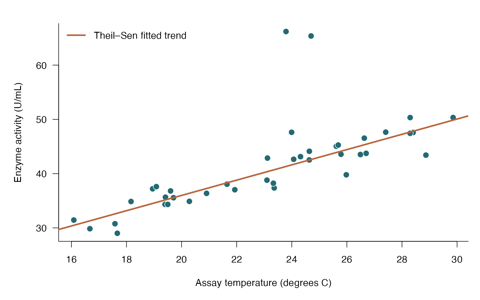
- Theil–Sen slope = 1.408 U/mL per degree C
- 95% pairs-bootstrap interval: 1.184 to 1.618
- Finite original pairwise slopes = 780; bootstrap replicates = 999
- The interval is approximate; no exact test p-value is reported.
The robust slope was 1.408 U/mL per degree C, with a 95% percentile pairs-bootstrap interval of 1.184 to 1.618 (999 replicates). This estimates a linear location trend resistant to extreme responses; its interval is approximate and is not an exact slope test.
**Teaching point:** A robust slope retains interpretable units while limiting extreme-response influence; uncertainty here is an approximate pairs-bootstrap interval.
### Analysis code excerpt
```r
d <- read.csv("modules/theil_sen/generated/data.csv")
pairs <- combn(seq_len(nrow(d)), 2)
slopes <- (d$activity[pairs[2, ]] - d$activity[pairs[1, ]]) /
(d$temp_c[pairs[2, ]] - d$temp_c[pairs[1, ]])
slope <- median(slopes)
intercept <- median(d$activity - slope * d$temp_c)
```
The full script supplies package loading and any additional preparation.
### Full printed R output
```text
intercept slope
7.832577 1.407600
2.5% 97.5%
1.183998 1.618227
[1] 999
```
### Recreate the observations
```r
output_dir <- "modules/theil_sen/generated"
dir.create(output_dir, recursive = TRUE, showWarnings = FALSE)
set.seed(1116)
temperature <- runif(40, 16, 30)
activity <- 8 + 1.4 * temperature + rt(40, df = 4) * 2
activity[c(5, 18)] <- activity[c(5, 18)] + 25
d <- data.frame(assay = 1:40, temp_c = temperature, activity = activity)
write.csv(d, file.path(output_dir, "data.csv"), row.names = FALSE)
```
Run the complete module from the course folder:
```sh
Rscript modules/theil_sen/analysis.R modules/theil_sen/generated
```
## Dataset 27: Exact binomial test
Host choice in a parasitoid wasp
**Family:** Proportions and categories · **Rows:** 80 · **Seed:** 3101
[Saved CSV](modules/binomial/generated/data.csv) · [Full runnable R script](modules/binomial/analysis.R) · [Full-size plot](modules/binomial/generated/plot.png)
**Generating truth:** The true native-host probability is 0.68, so the null probability 0.50 is false. The population difference from the null is +0.18.
**Exact generating model:** Generate 80 independent Bernoulli choices, each with probability 0.68 of a native-host choice. Each wasp appears once. No rounding or dependence is introduced.
**Scientific question:** Do wasps choose the native host with probability 0.50?
**Null being tested / estimation target:** The population probability of choosing the native host is 0.50.
**Design and independent unit:** One independent choice per wasp; two equally available host species.
### Columns
| Column | Meaning | Unit / type |
|---|---|---|
| wasp | Unique independent wasp identifier | none |
| native | 1 = native host chosen; 0 = introduced host | binary |
### Analysis from the saved dataset
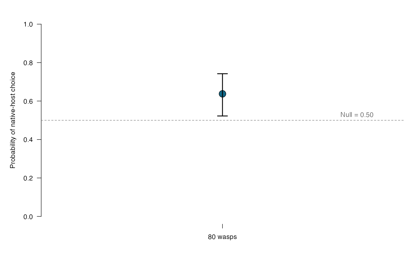
- Native-host choices: 51 / 80
- Estimated probability: 0.637
- 95% exact CI: 0.522 to 0.742
- Exact two-sided p = 0.01832
Native-host choice was 63.7% (95% exact CI 52.2–74.2%; p = 0.0183 against 50%). This estimates preference under the simulated choice conditions.
**Teaching point:** The null probability comes from the scientific prediction, not automatically from the fact that there are two outcomes.
### Analysis code excerpt
```r
d <- read.csv("modules/binomial/generated/data.csv")
x <- sum(d$native)
fit <- binom.test(x, nrow(d), p = 0.5,
alternative = "two.sided")
estimate <- x / nrow(d)
ci <- fit$conf.int
```
The full script supplies package loading and any additional preparation.
### Full printed R output
```text
Exact binomial test
data: x and nrow(d)
number of successes = 51, number of trials = 80, p-value = 0.01832
alternative hypothesis: true probability of success is not equal to 0.5
95 percent confidence interval:
0.5223873 0.7421051
sample estimates:
probability of success
0.6375
```
### Recreate the observations
```r
out_dir <- "modules/binomial/generated"
dir.create(out_dir, recursive = TRUE, showWarnings = FALSE)
set.seed(3101)
d <- data.frame(wasp = 1:80,
native = rbinom(80, 1, 0.68))
write.csv(d, file.path(out_dir, "data.csv"), row.names = FALSE)
```
Run the complete module from the course folder:
```sh
Rscript modules/binomial/analysis.R modules/binomial/generated
```
## Dataset 28: One-proportion test
Germination of salt-tolerant seeds
**Family:** Proportions and categories · **Rows:** 120 · **Seed:** 3102
[Saved CSV](modules/one_proportion/generated/data.csv) · [Full runnable R script](modules/one_proportion/analysis.R) · [Full-size plot](modules/one_proportion/generated/plot.png)
**Generating truth:** The true germination probability is 0.67 rather than the null benchmark 0.50; the population difference is +0.17.
**Exact generating model:** Generate 120 independent seeds with Bernoulli germination probability 0.67. Every seed has the same probability. No rounding or tray dependence is simulated.
**Scientific question:** Does the germination probability differ from the 50% benchmark?
**Null being tested / estimation target:** The population germination probability is 0.50.
**Design and independent unit:** One germination outcome per seed under a fixed salt treatment.
### Columns
| Column | Meaning | Unit / type |
|---|---|---|
| seed | Unique independent seed identifier | none |
| germinated | 1 = germinated; 0 = did not germinate | binary |
### Analysis from the saved dataset
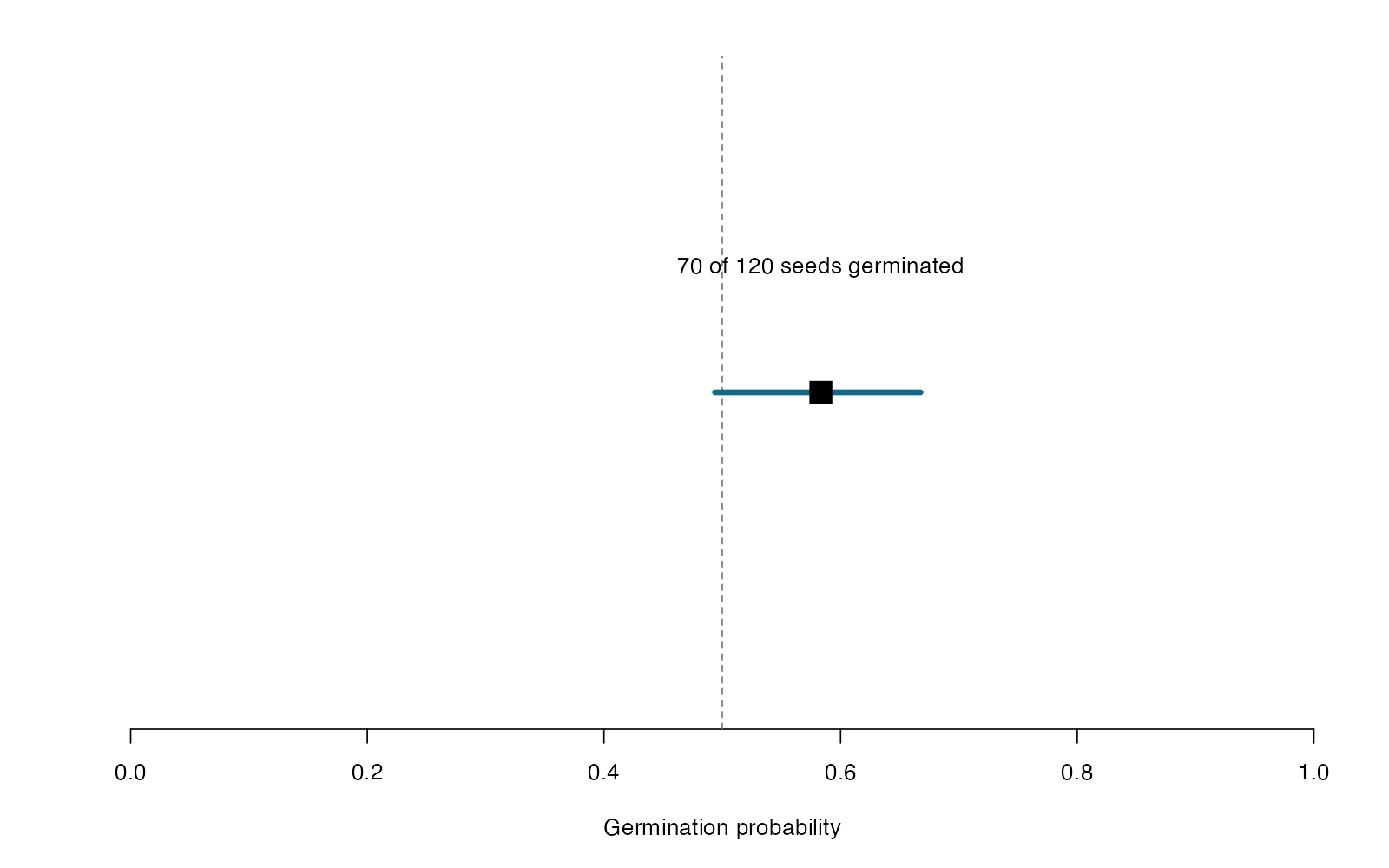
- Germination: 70 / 120
- Estimated probability: 0.583
- 95% score CI: 0.494 to 0.668
- Two-sided p = 0.06789
Germination was 58.3% (95% score CI 49.4–66.8%; p = 0.0679 against 50%). The test concerns this germination probability, not the mean of arbitrary continuous percentages.
**Teaching point:** A binomial proportion is successes out of a known number of trials; arbitrary continuous percentages are different data.
### Analysis code excerpt
```r
d <- read.csv("modules/one_proportion/generated/data.csv")
x <- sum(d$germinated)
fit <- prop.test(x, nrow(d), p = 0.5,
alternative = "two.sided", correct = FALSE)
estimate <- x / nrow(d)
ci <- fit$conf.int
```
The full script supplies package loading and any additional preparation.
### Full printed R output
```text
1-sample proportions test without continuity correction
data: x out of nrow(d), null probability 0.5
X-squared = 3.3333, df = 1, p-value = 0.06789
alternative hypothesis: true p is not equal to 0.5
95 percent confidence interval:
0.4938803 0.6676165
sample estimates:
p
0.5833333
```
### Recreate the observations
```r
out_dir <- "modules/one_proportion/generated"
dir.create(out_dir, recursive = TRUE, showWarnings = FALSE)
set.seed(3102)
d <- data.frame(seed = 1:120,
germinated = rbinom(120, 1, 0.67))
write.csv(d, file.path(out_dir, "data.csv"), row.names = FALSE)
```
Run the complete module from the course folder:
```sh
Rscript modules/one_proportion/analysis.R modules/one_proportion/generated
```
## Dataset 29: Two-proportion test
Heat survival in evolved and ancestral yeast
**Family:** Proportions and categories · **Rows:** 220 · **Seed:** 3103
[Saved CSV](modules/two_proportions/generated/data.csv) · [Full runnable R script](modules/two_proportions/analysis.R) · [Full-size plot](modules/two_proportions/generated/plot.png)
**Generating truth:** Evolved minus ancestral survival probability is 0.20, so the equal-probabilities null is false. The corresponding population odds ratio is approximately 2.37.
**Exact generating model:** Generate 110 independent evolved cultures and 110 independent ancestral cultures. Survival is Bernoulli with probabilities 0.72 and 0.52, respectively. No batching or pairing is introduced.
**Scientific question:** Does survival probability differ between evolved and ancestral yeast?
**Null being tested / estimation target:** Evolved and ancestral cultures have equal survival probabilities.
**Design and independent unit:** Independent cultures assigned to one genotype; survival is scored once.
### Columns
| Column | Meaning | Unit / type |
|---|---|---|
| group | Culture genotype: Evolved or Ancestral | none |
| survived | 1 = survived heat; 0 = died | binary |
### Analysis from the saved dataset
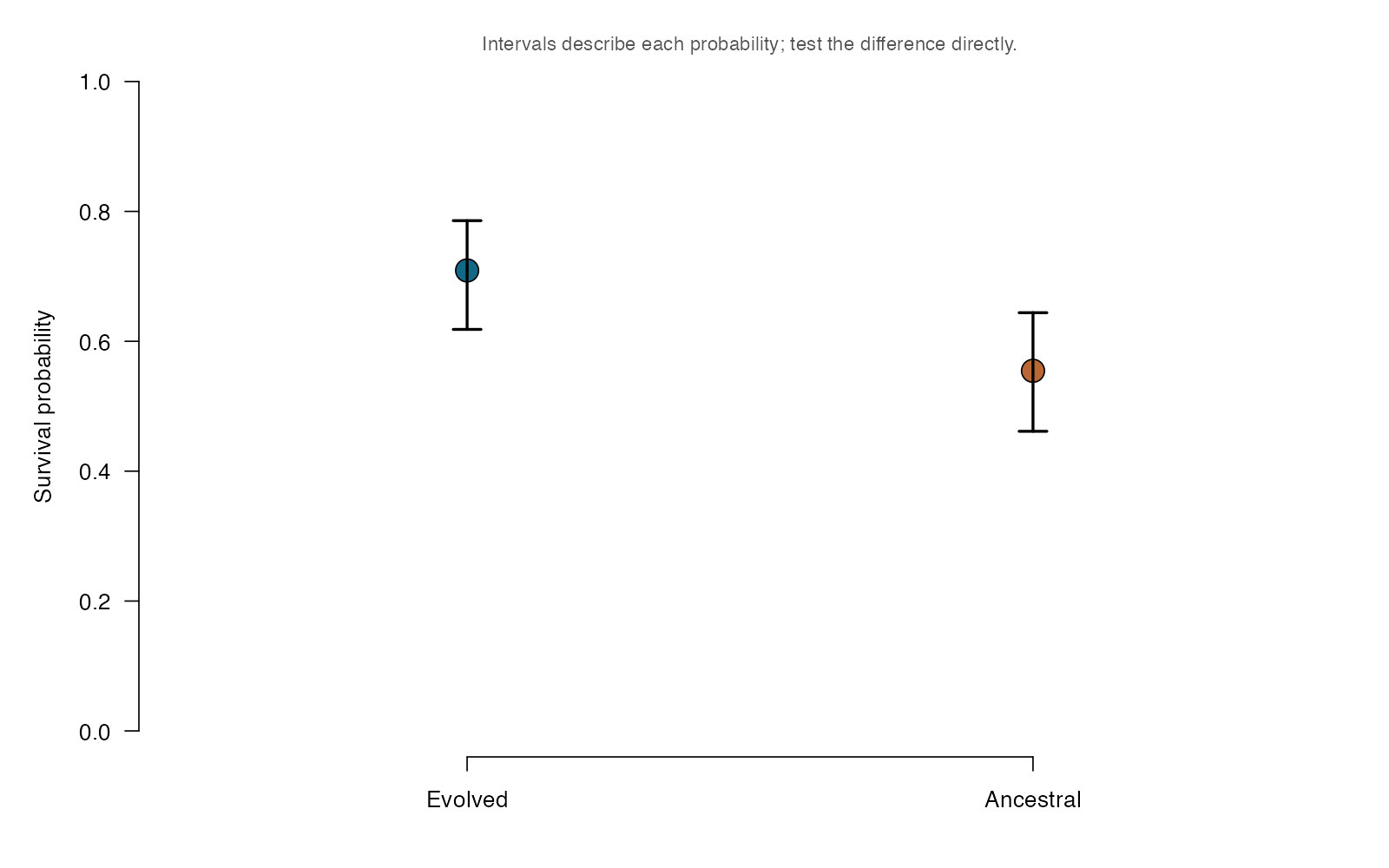
- Evolved: 78 / 110; ancestral: 61 / 110
- Difference (evolved − ancestral): 0.155
- 95% CI for difference: 0.029 to 0.280
- Two-sided p = 0.01748
Evolved minus ancestral survival was 15.5 percentage points (95% CI 2.9 to 28.0; p = 0.0175). The interval for this difference answers the comparison directly.
**Teaching point:** Keep group order explicit: the contrast is evolved minus ancestral, and its confidence interval addresses the actual comparison.
### Analysis code excerpt
```r
d <- read.csv("modules/two_proportions/generated/data.csv")
groups <- c("Evolved", "Ancestral")
x <- sapply(groups, function(g) sum(d$survived[d$group == g]))
n <- sapply(groups, function(g) sum(d$group == g))
fit <- prop.test(x, n, correct = FALSE)
estimate <- x / n
difference <- estimate[1] - estimate[2]
ci <- fit$conf.int
group_ci <- sapply(1:2, function(i) prop.test(x[i], n[i],
correct = FALSE)$conf.int)
```
The full script supplies package loading and any additional preparation.
### Full printed R output
```text
2-sample test for equality of proportions without continuity correction
data: x out of n
X-squared = 5.647, df = 1, p-value = 0.01748
alternative hypothesis: two.sided
95 percent confidence interval:
0.02872612 0.28036479
sample estimates:
prop 1 prop 2
0.7090909 0.5545455
```
### Recreate the observations
```r
out_dir <- "modules/two_proportions/generated"
dir.create(out_dir, recursive = TRUE, showWarnings = FALSE)
set.seed(3103)
d <- data.frame(group = rep(c("Evolved", "Ancestral"), each = 110))
d$survived <- rbinom(220, 1, rep(c(.72, .52), each = 110))
write.csv(d, file.path(out_dir, "data.csv"), row.names = FALSE)
```
Run the complete module from the course folder:
```sh
Rscript modules/two_proportions/analysis.R modules/two_proportions/generated
```
## Dataset 30: Chi-square goodness-of-fit
Segregation in an F2 cross
**Family:** Proportions and categories · **Rows:** 240 · **Seed:** 3104
[Saved CSV](modules/chi_gof/generated/data.csv) · [Full runnable R script](modules/chi_gof/analysis.R) · [Full-size plot](modules/chi_gof/generated/plot.png)
**Generating truth:** The simulated probabilities differ from 1:2:1 by -0.07, +0.04, and +0.03. The goodness-of-fit null is false.
**Exact generating model:** Independently sample 240 offspring genotypes with probabilities AA = 0.18, Aa = 0.54, aa = 0.28. Test against the fixed Mendelian probabilities 0.25, 0.50, 0.25; no probabilities are estimated for the null.
**Scientific question:** Do the genotype frequencies follow the expected 1:2:1 segregation ratio?
**Null being tested / estimation target:** Genotype probabilities are AA = 0.25, Aa = 0.50, and aa = 0.25.
**Design and independent unit:** Each offspring is assigned to one of three genotypes.
### Columns
| Column | Meaning | Unit / type |
|---|---|---|
| offspring | Unique independent offspring identifier | none |
| genotype | AA, Aa, or aa genotype category | none |
### Analysis from the saved dataset
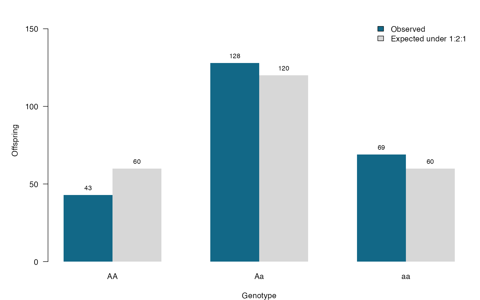
- Observed: 43, 128, 69
- Expected: 60, 120, 60
- Chi-square = 6.700; df = 2
- p = 0.03508
Observed genotype proportions were 0.179, 0.533, 0.287. The goodness-of-fit test gives chi-square(2) = 6.70, p = 0.0351 against the prespecified 1:2:1 ratio; the test does not identify a biological mechanism for the departure.
**Teaching point:** Expected counts encode the biological hypothesis. Equal expected counts would test a different hypothesis.
### Analysis code excerpt
```r
d <- read.csv("modules/chi_gof/generated/data.csv")
observed <- table(factor(d$genotype, levels = c("AA", "Aa", "aa")))
fit <- chisq.test(observed, p = c(.25, .50, .25))
expected <- as.numeric(fit$expected)
departures <- observed / sum(observed) - c(.25, .50, .25)
```
The full script supplies package loading and any additional preparation.
### Full printed R output
```text
Chi-squared test for given probabilities
data: observed
X-squared = 6.7, df = 2, p-value = 0.03508
```
### Recreate the observations
```r
out_dir <- "modules/chi_gof/generated"
dir.create(out_dir, recursive = TRUE, showWarnings = FALSE)
set.seed(3104)
d <- data.frame(offspring = 1:240,
genotype = sample(c("AA", "Aa", "aa"), 240, replace = TRUE,
prob = c(.18, .54, .28)))
write.csv(d, file.path(out_dir, "data.csv"), row.names = FALSE)
```
Run the complete module from the course folder:
```sh
Rscript modules/chi_gof/analysis.R modules/chi_gof/generated
```
## Dataset 31: Chi-square test of independence
Infection across three lizard habitats
**Family:** Proportions and categories · **Rows:** 270 · **Seed:** 3105
[Saved CSV](modules/chi_independence/generated/data.csv) · [Full runnable R script](modules/chi_independence/analysis.R) · [Full-size plot](modules/chi_independence/generated/plot.png)
**Generating truth:** Infection probability depends on habitat, so the independence null is false. Urban minus forest infection probability is 0.30; the simulation does not assign causality to habitat.
**Exact generating model:** Generate 90 independent lizards from each of Forest, Grassland, and Urban habitats. Infection is Bernoulli with probabilities 0.25, 0.42, and 0.55, respectively. No site-level clustering is simulated.
**Scientific question:** Is infection status associated with habitat?
**Null being tested / estimation target:** Infection status and habitat are independent; infection probabilities are equal across habitats.
**Design and independent unit:** Independent lizards sampled once in one of three habitats.
### Columns
| Column | Meaning | Unit / type |
|---|---|---|
| habitat | Sampling habitat: Forest, Grassland, or Urban | none |
| infection | Infected or Uninfected status | none |
### Analysis from the saved dataset
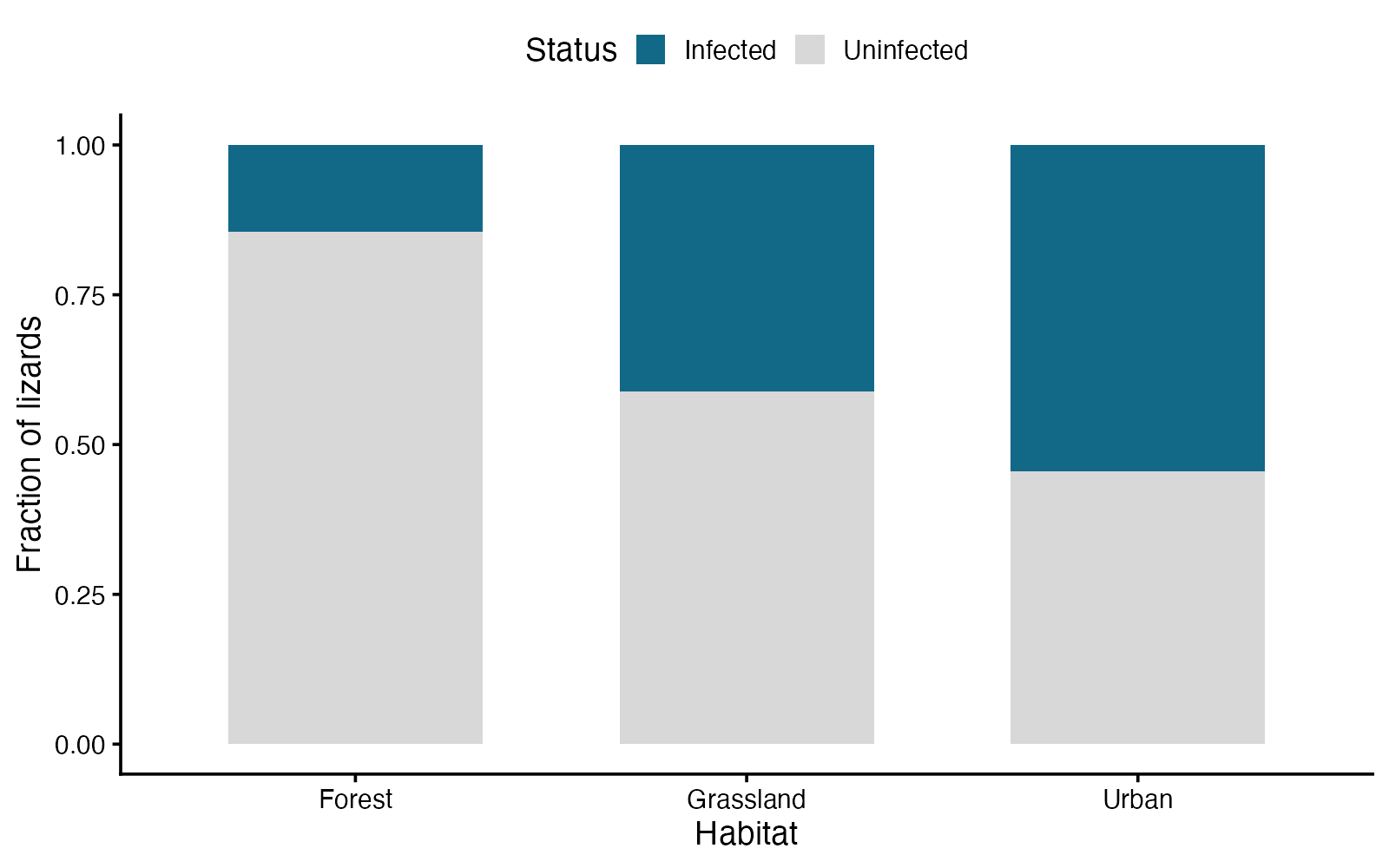
- Infection probabilities: Forest 0.14; Grassland 0.41; Urban 0.54
- Minimum expected count: 33.0
- Chi-square(2) = 32.153
- p = 1.042e-07; Cramer V = 0.345
Infection probabilities differed descriptively across habitats (Forest 14%, Grassland 41%, Urban 54%). The independence test gives chi-square(2) = 32.15, p = 1.04e-07; Cramer V = 0.35. This observational association does not establish a habitat effect.
**Teaching point:** A significant omnibus association does not establish a causal habitat effect or identify every differing pair.
### Analysis code excerpt
```r
d <- read.csv("modules/chi_independence/generated/data.csv")
tab <- table(d$habitat, d$infection)
fit <- chisq.test(tab, correct = FALSE)
cramers_v <- sqrt(as.numeric(fit$statistic) /
(sum(tab) * min(nrow(tab)-1, ncol(tab)-1)))
rates <- prop.table(tab, 1)[, "Infected"]
```
The full script supplies package loading and any additional preparation.
### Full printed R output
```text
Pearson's Chi-squared test
data: tab
X-squared = 32.153, df = 2, p-value = 1.042e-07
```
### Recreate the observations
```r
out_dir <- "modules/chi_independence/generated"
dir.create(out_dir, recursive = TRUE, showWarnings = FALSE)
set.seed(3105)
d <- data.frame(habitat = rep(c("Forest", "Grassland", "Urban"), each = 90))
d$infection <- ifelse(rbinom(270, 1, rep(c(.25, .42, .55), each = 90)),
"Infected", "Uninfected")
write.csv(d, file.path(out_dir, "data.csv"), row.names = FALSE)
```
Run the complete module from the course folder:
```sh
Rscript modules/chi_independence/analysis.R modules/chi_independence/generated
```
## Dataset 32: Fisher exact test
Survival of rare resistant and susceptible clones
**Family:** Proportions and categories · **Rows:** 24 · **Seed:** 3106
[Saved CSV](modules/fisher_exact/generated/data.csv) · [Full runnable R script](modules/fisher_exact/analysis.R) · [Full-size plot](modules/fisher_exact/generated/plot.png)
**Generating truth:** The resistant-to-susceptible population survival odds ratio is (0.65/0.35)/(0.20/0.80), approximately 7.43. The odds-ratio-one null is false.
**Exact generating model:** Generate 12 independent susceptible clones with survival probability 0.20 and 12 independent resistant clones with probability 0.65. Each contributes one Bernoulli outcome; small table cells are intentional.
**Scientific question:** Are survival odds associated with clone type?
**Null being tested / estimation target:** The population odds ratio for clone type and survival is 1.
**Design and independent unit:** Two small independent clone groups; binary survival after exposure.
### Columns
| Column | Meaning | Unit / type |
|---|---|---|
| clone | Unique independent clone identifier | none |
| type | Susceptible or Resistant clone type | none |
| survived | 1 = survived exposure; 0 = died | binary |
### Analysis from the saved dataset
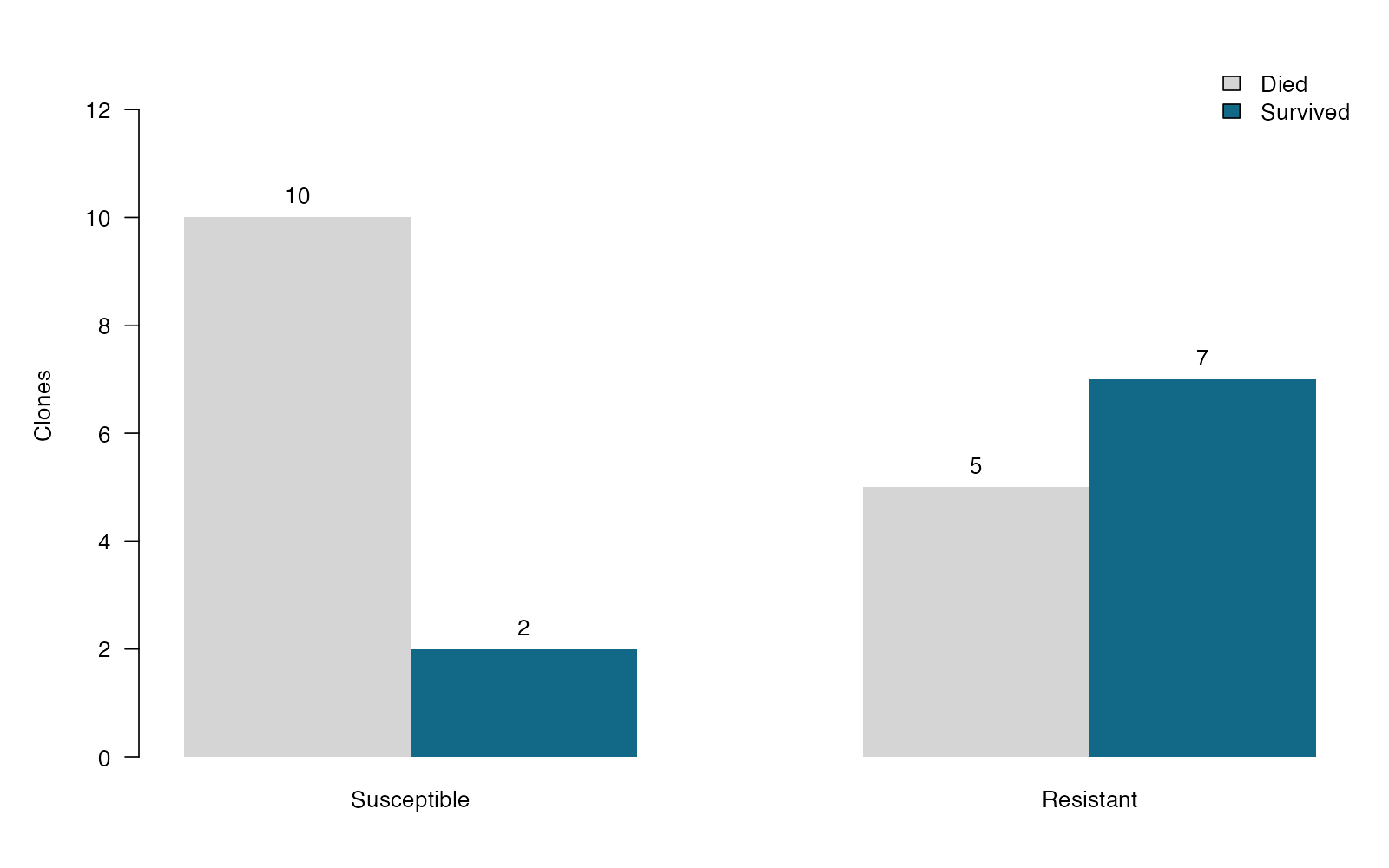
- Survivors: susceptible 2/12; resistant 7/12
- Survival odds ratio (resistant / susceptible): 6.395
- 95% exact CI: 0.810 to 85.671
- Two-sided exact p = 0.08938
The resistant-to-susceptible survival odds ratio was 6.39 (95% exact CI 0.81–85.67; p = 0.0894). A wide interval reflects limited information from these small groups; odds are not probabilities.
**Teaching point:** Exact inference handles sparse counts, but it cannot create the precision missing from a small sample.
### Analysis code excerpt
```r
d <- read.csv("modules/fisher_exact/generated/data.csv")
tab <- table(factor(d$type, levels = c("Susceptible", "Resistant")),
factor(d$survived, levels = c(0, 1)))
fit <- fisher.test(tab, alternative = "two.sided")
odds_ratio <- unname(fit$estimate)
ci <- fit$conf.int
```
The full script supplies package loading and any additional preparation.
### Full printed R output
```text
Fisher's Exact Test for Count Data
data: tab
p-value = 0.08938
alternative hypothesis: true odds ratio is not equal to 1
95 percent confidence interval:
0.8098091 85.6709653
sample estimates:
odds ratio
6.394505
```
### Recreate the observations
```r
out_dir <- "modules/fisher_exact/generated"
dir.create(out_dir, recursive = TRUE, showWarnings = FALSE)
set.seed(3106)
d <- data.frame(clone = 1:24,
type = rep(c("Susceptible", "Resistant"), each = 12))
d$survived <- rbinom(24, 1, rep(c(.20, .65), each = 12))
write.csv(d, file.path(out_dir, "data.csv"), row.names = FALSE)
```
Run the complete module from the course folder:
```sh
Rscript modules/fisher_exact/analysis.R modules/fisher_exact/generated
```
## Dataset 33: McNemar test
Antibody detection before and after an exposure season
**Family:** Paired binary outcomes · **Rows:** 80 · **Seed:** 3107
[Saved CSV](modules/mcnemar/generated/data.csv) · [Full runnable R script](modules/mcnemar/analysis.R) · [Full-size plot](modules/mcnemar/generated/plot.png)
**Generating truth:** Marginal after positivity is 0.45×0.85 + 0.55×0.35 = 0.575, a +0.125 change from before. Population gain and loss probabilities are 0.1925 and 0.0675, so the McNemar null is false.
**Exact generating model:** Generate 80 independent mice. Before status is Bernoulli(0.45). Conditional after positivity is 0.85 for a previously positive mouse and 0.35 for a previously negative mouse, producing correlated within-mouse measurements.
**Scientific question:** Does the marginal probability of antibody detection change between visits?
**Null being tested / estimation target:** The probability of changing from negative to positive equals that of changing from positive to negative.
**Design and independent unit:** The same 80 wild mice are sampled twice.
### Columns
| Column | Meaning | Unit / type |
|---|---|---|
| mouse | Matched mouse identifier | none |
| before | Antibody detected at the first visit (1 = yes) | binary |
| after | Antibody detected at the second visit (1 = yes) | binary |
### Analysis from the saved dataset
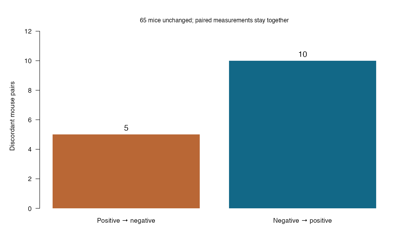
- Gained detection: 10; lost detection: 5
- Before: 0.438; after: 0.500
- Change: 0.062
- McNemar p = 0.1967; exact paired p = 0.3018
Detection changed from 43.8% to 50.0% (change 6.2 percentage points). There were 10 gains and 5 losses; McNemar p = 0.197 and exact paired p = 0.302. The comparison preserves mouse identity.
**Teaching point:** The information about a change is in discordant pairs. Keeping the mouse identity changes the appropriate test.
### Analysis code excerpt
```r
d <- read.csv("modules/mcnemar/generated/data.csv")
tab <- table(factor(d$before, levels = 0:1),
factor(d$after, levels = 0:1))
fit <- mcnemar.test(tab, correct = FALSE)
gained <- tab[1, 2]
lost <- tab[2, 1]
exact <- binom.test(gained, gained + lost, p = .5)
change <- mean(d$after) - mean(d$before)
```
The full script supplies package loading and any additional preparation.
### Full printed R output
```text
$McNemar
McNemar's Chi-squared test
data: tab
McNemar's chi-squared = 1.6667, df = 1, p-value = 0.1967
$exact_discordant_pairs
Exact binomial test
data: gained and gained + lost
number of successes = 10, number of trials = 15, p-value = 0.3018
alternative hypothesis: true probability of success is not equal to 0.5
95 percent confidence interval:
0.3838037 0.8817589
sample estimates:
probability of success
0.6666667
```
### Recreate the observations
```r
out_dir <- "modules/mcnemar/generated"
dir.create(out_dir, recursive = TRUE, showWarnings = FALSE)
set.seed(3107)
d <- data.frame(mouse = 1:80, before = rbinom(80, 1, .45))
d$after <- rbinom(80, 1, ifelse(d$before == 1, .85, .35))
write.csv(d, file.path(out_dir, "data.csv"), row.names = FALSE)
```
Run the complete module from the course folder:
```sh
Rscript modules/mcnemar/analysis.R modules/mcnemar/generated
```
## Dataset 34: Cochran’s Q test
Bee visits to three floral odors
**Family:** Paired binary outcomes · **Rows:** 180 · **Seed:** 3108
[Saved CSV](modules/cochran_q/generated/data.csv) · [Full runnable R script](modules/cochran_q/analysis.R) · [Full-size plot](modules/cochran_q/generated/plot.png)
**Generating truth:** Increasing odor effects produce strictly increasing marginal visit probabilities across A, B, and C. The equal-probabilities null is false; the latent log-odds differences are not themselves the marginal probability differences.
**Exact generating model:** Generate 60 independent bees, each with a Normal(0, 0.8²) latent effect. Each bee encounters odors A, B, and C. Visit logits are -0.7 + bee effect + odor effect, with odor effects 0, 0.5, and 1. Outcomes are independent conditional on the bee effect but correlated within a bee marginally.
**Scientific question:** Are marginal visit probabilities equal for all three odors?
**Null being tested / estimation target:** The three odor conditions have equal marginal probabilities of a visit.
**Design and independent unit:** Each bee experiences all odors in randomized sessions with a washout.
### Columns
| Column | Meaning | Unit / type |
|---|---|---|
| bee | Independent bee and repeated-measures identifier | none |
| odor | Repeated odor condition: A, B, or C | none |
| visit | 1 = visit; 0 = no visit | binary |
### Analysis from the saved dataset
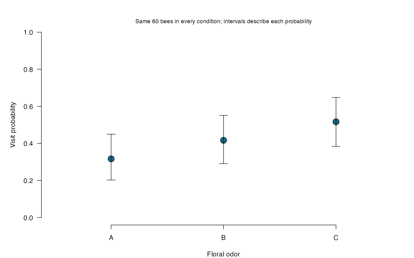
- Matched bees: 60; conditions: 3
- Visit probabilities: 0.317, 0.417, 0.517
- Q = 5.143; df = 2
- Omnibus p = 0.07643
Visit probabilities were 31.7%, 41.7%, 51.7%. Cochran Q(2) = 5.14, p = 0.0764 tests equality across all odors while retaining matching. It does not identify which odor pairs differ.
**Teaching point:** A matched omnibus binary test uses complete sets of responses; a significant result does not identify which conditions differ.
### Analysis code excerpt
```r
d <- read.csv("modules/cochran_q/generated/data.csv")
wide <- xtabs(visit ~ bee + odor, data = d)
k <- ncol(wide)
C <- colSums(wide)
R <- rowSums(wide)
Q <- (k - 1) * (k * sum(C^2) - sum(C)^2) /
(k * sum(R) - sum(R^2))
p_value <- pchisq(Q, df = k - 1, lower.tail = FALSE)
rates <- C / nrow(wide)
ci <- sapply(1:k, function(j) binom.test(C[j], nrow(wide))$conf.int)
```
The full script supplies package loading and any additional preparation.
### Full printed R output
```text
$statistic
[1] 5.142857
$df
[1] 2
$p.value
[1] 0.07642629
$visit_probabilities
A B C
0.3166667 0.4166667 0.5166667
```
### Recreate the observations
```r
out_dir <- "modules/cochran_q/generated"
dir.create(out_dir, recursive = TRUE, showWarnings = FALSE)
set.seed(3108)
bee_effect <- rnorm(60, 0, .8)
d <- data.frame(bee = rep(1:60, each = 3),
odor = rep(c("A", "B", "C"), 60))
d$visit <- rbinom(180, 1,
plogis(-.7 + rep(bee_effect, each = 3) + rep(c(0, .5, 1), 60)))
write.csv(d, file.path(out_dir, "data.csv"), row.names = FALSE)
```
Run the complete module from the course folder:
```sh
Rscript modules/cochran_q/analysis.R modules/cochran_q/generated
```
## Dataset 35: Logistic regression
Hybrid viability across parental divergence
**Family:** Generalized linear models · **Rows:** 160 · **Seed:** 3110
[Saved CSV](modules/logistic/generated/data.csv) · [Full runnable R script](modules/logistic/analysis.R) · [Full-size plot](modules/logistic/generated/plot.png)
**Generating truth:** The true divergence coefficient is -0.5; viability odds are multiplied by exp(-0.5) ≈ 0.607 per divergence percentage point. The zero-slope null is false. The probability decline is nonlinear.
**Exact generating model:** Generate 160 independent crosses with divergence Uniform(0,8) percentage points. One hybrid viability outcome per cross is Bernoulli with probability plogis(1.9 - 0.5 × divergence). Predictors are not rounded.
**Scientific question:** Does viability probability change with parental divergence?
**Null being tested / estimation target:** The divergence coefficient is zero: modeled viability odds do not change with divergence.
**Design and independent unit:** One independent hybrid offspring per cross.
### Columns
| Column | Meaning | Unit / type |
|---|---|---|
| cross | Unique independent cross identifier | none |
| divergence | Parental divergence | percentage points |
| viable | 1 = viable hybrid; 0 = nonviable | binary |
### Analysis from the saved dataset
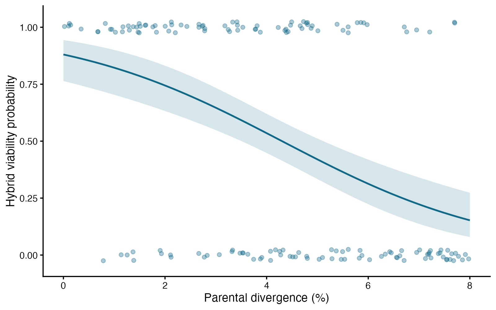
- Divergence coefficient: -0.464
- Odds ratio per percentage point: 0.629
- 95% Wald CI for odds ratio: 0.528 to 0.749
- Likelihood-ratio p = 6.573e-09
Each additional percentage point of divergence multiplied modeled viability odds by 0.63 (95% Wald CI 0.53–0.75; likelihood-ratio p = 6.57e-09). The curve translates odds into probabilities; this association alone does not establish causation.
**Teaching point:** A coefficient describes log odds; translate to odds ratios or plotted probabilities to answer the biological question.
### Analysis code excerpt
```r
d <- read.csv("modules/logistic/generated/data.csv")
fit <- glm(viable ~ divergence, data = d, family = binomial)
test <- drop1(fit, test = "Chisq")
p_value <- test["divergence", "Pr(>Chi)"]
b <- coef(fit)["divergence"]
se <- sqrt(vcov(fit)["divergence", "divergence"])
odds_ratio <- exp(b)
ci <- exp(b + c(-1, 1) * 1.96 * se)
```
The full script supplies package loading and any additional preparation.
### Full printed R output
```text
Call:
glm(formula = viable ~ divergence, family = binomial, data = d)
Coefficients:
Estimate Std. Error z value Pr(>|z|)
(Intercept) 1.99600 0.41934 4.760 1.94e-06 ***
divergence -0.46382 0.08915 -5.203 1.96e-07 ***
---
Signif. codes: 0 ‘***’ 0.001 ‘**’ 0.01 ‘*’ 0.05 ‘.’ 0.1 ‘ ’ 1
(Dispersion parameter for binomial family taken to be 1)
Null deviance: 221.78 on 159 degrees of freedom
Residual deviance: 188.12 on 158 degrees of freedom
AIC: 192.12
Number of Fisher Scoring iterations: 4
```
### Recreate the observations
```r
out_dir <- "modules/logistic/generated"
dir.create(out_dir, recursive = TRUE, showWarnings = FALSE)
set.seed(3110)
d <- data.frame(cross = 1:160, divergence = runif(160, 0, 8))
d$viable <- rbinom(160, 1, plogis(1.9 - .5 * d$divergence))
write.csv(d, file.path(out_dir, "data.csv"), row.names = FALSE)
```
Run the complete module from the course folder:
```sh
Rscript modules/logistic/analysis.R modules/logistic/generated
```
## Dataset 36: Exact Poisson rate test
De novo mutations in sequenced microbial lineages
**Family:** Counts and exposure · **Rows:** 60 · **Seed:** 3109
[Saved CSV](modules/poisson_exact/generated/data.csv) · [Full runnable R script](modules/poisson_exact/analysis.R) · [Full-size plot](modules/poisson_exact/generated/plot.png)
**Generating truth:** The true rate is 0.40 mutations/Mb rather than the null rate 0.25/Mb. The population rate ratio to the null is 1.6.
**Exact generating model:** Generate 60 independent lineages with callable sequence Uniform(8,20) megabases. Each count is Poisson with mean 0.40 × callable megabases. The population rate is constant across lineages and exposure is unrounded.
**Scientific question:** Does the mutation rate differ from 0.25 mutations per callable megabase?
**Null being tested / estimation target:** The common mutation rate is 0.25 per callable megabase.
**Design and independent unit:** Independent lineages have different amounts of callable sequence.
### Columns
| Column | Meaning | Unit / type |
|---|---|---|
| lineage | Unique independent microbial lineage | none |
| megabases | Callable sequence exposure | Mb |
| mutations | Observed de novo mutations | count |
### Analysis from the saved dataset
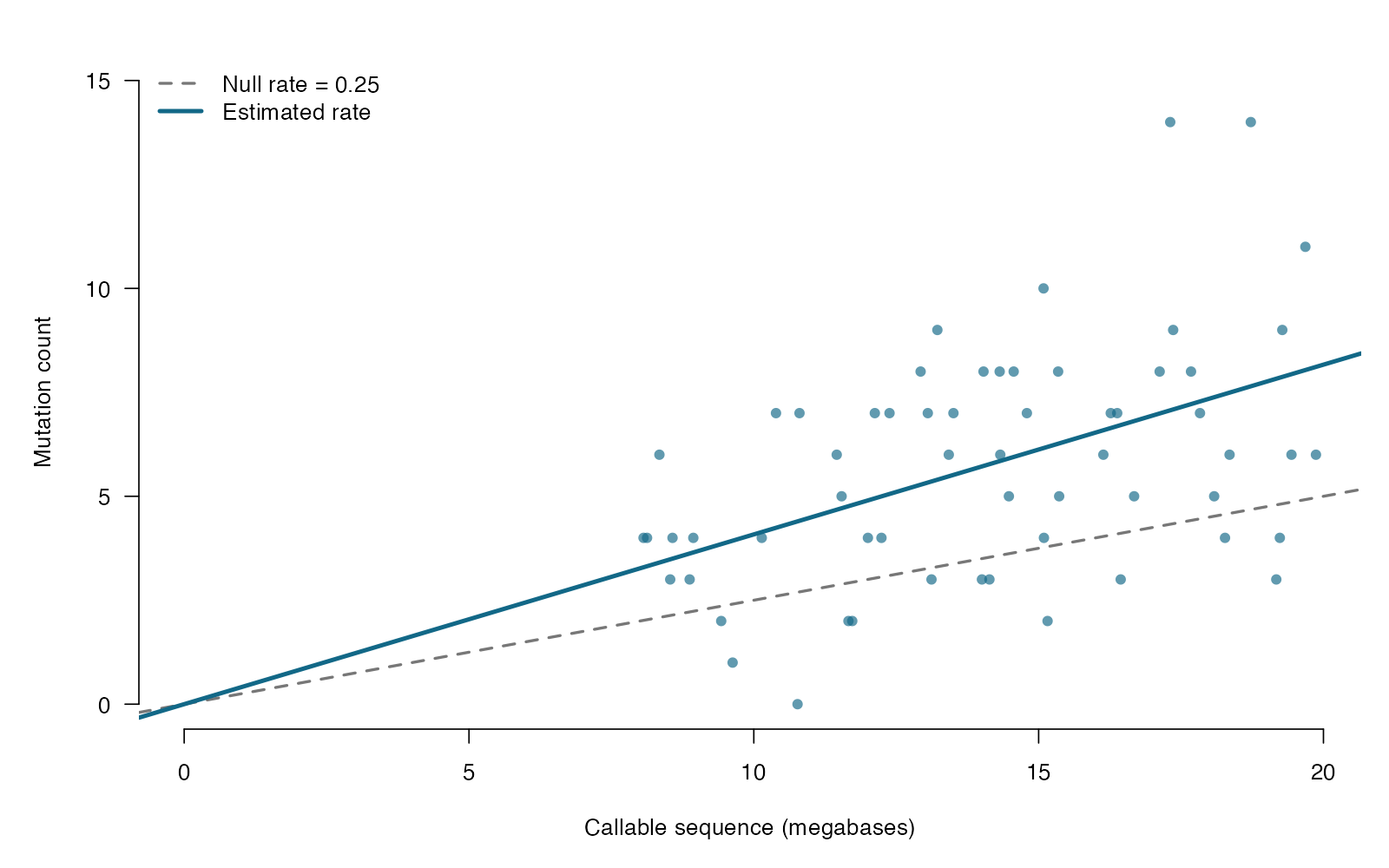
- Events: 345; exposure: 845.0 Mb
- Rate: 0.408 mutations/Mb
- 95% exact CI: 0.366 to 0.454
- Exact p = 3.246e-17
The mutation rate was 0.408 per callable Mb (95% exact CI 0.366–0.454; p = 3.25e-17 against 0.25/Mb). Pooling counts is justified here by the common-rate Poisson model.
**Teaching point:** A count becomes a rate only after the exposure and its units are supplied.
### Analysis code excerpt
```r
d <- read.csv("modules/poisson_exact/generated/data.csv")
fit <- poisson.test(sum(d$mutations), T = sum(d$megabases),
r = .25, alternative = "two.sided")
rate <- sum(d$mutations) / sum(d$megabases)
ci <- fit$conf.int
```
The full script supplies package loading and any additional preparation.
### Full printed R output
```text
Exact Poisson test
data: sum(d$mutations) time base: sum(d$megabases)
number of events = 345, time base = 844.99, p-value < 2.2e-16
alternative hypothesis: true event rate is not equal to 0.25
95 percent confidence interval:
0.3663373 0.4537273
sample estimates:
event rate
0.4082887
```
### Recreate the observations
```r
out_dir <- "modules/poisson_exact/generated"
dir.create(out_dir, recursive = TRUE, showWarnings = FALSE)
set.seed(3109)
d <- data.frame(lineage = 1:60, megabases = runif(60, 8, 20))
d$mutations <- rpois(60, .40 * d$megabases)
write.csv(d, file.path(out_dir, "data.csv"), row.names = FALSE)
```
Run the complete module from the course folder:
```sh
Rscript modules/poisson_exact/analysis.R modules/poisson_exact/generated
```
## Dataset 37: Poisson regression
Coral recruit counts and live coral cover
**Family:** Generalized linear models · **Rows:** 120 · **Seed:** 3111
[Saved CSV](modules/poisson_glm/generated/data.csv) · [Full runnable R script](modules/poisson_glm/analysis.R) · [Full-size plot](modules/poisson_glm/generated/plot.png)
**Generating truth:** The true cover coefficient is 0.016. A 10-point cover increase multiplies recruit density by exp(0.16) ≈ 1.174. The zero-slope null is false, and the exposure coefficient is fixed at one.
**Exact generating model:** Generate 120 independent transects. Cover is Uniform(0,80) percentage points and area is independently Uniform(2,8) square meters. Recruit counts are Poisson(area × exp(-0.5 + 0.016 × cover)). No clustering or rounding is introduced.
**Scientific question:** Does recruit density change with live coral cover after accounting for surveyed area?
**Null being tested / estimation target:** The coral-cover coefficient is zero: recruit rate per square meter is unrelated to cover in this model.
**Design and independent unit:** Independent transects differ in surveyed area and live coral cover.
### Columns
| Column | Meaning | Unit / type |
|---|---|---|
| transect | Unique independent transect identifier | none |
| cover | Live coral cover | percentage points |
| area | Surveyed transect area | m² |
| recruits | Observed coral recruits | count |
### Analysis from the saved dataset
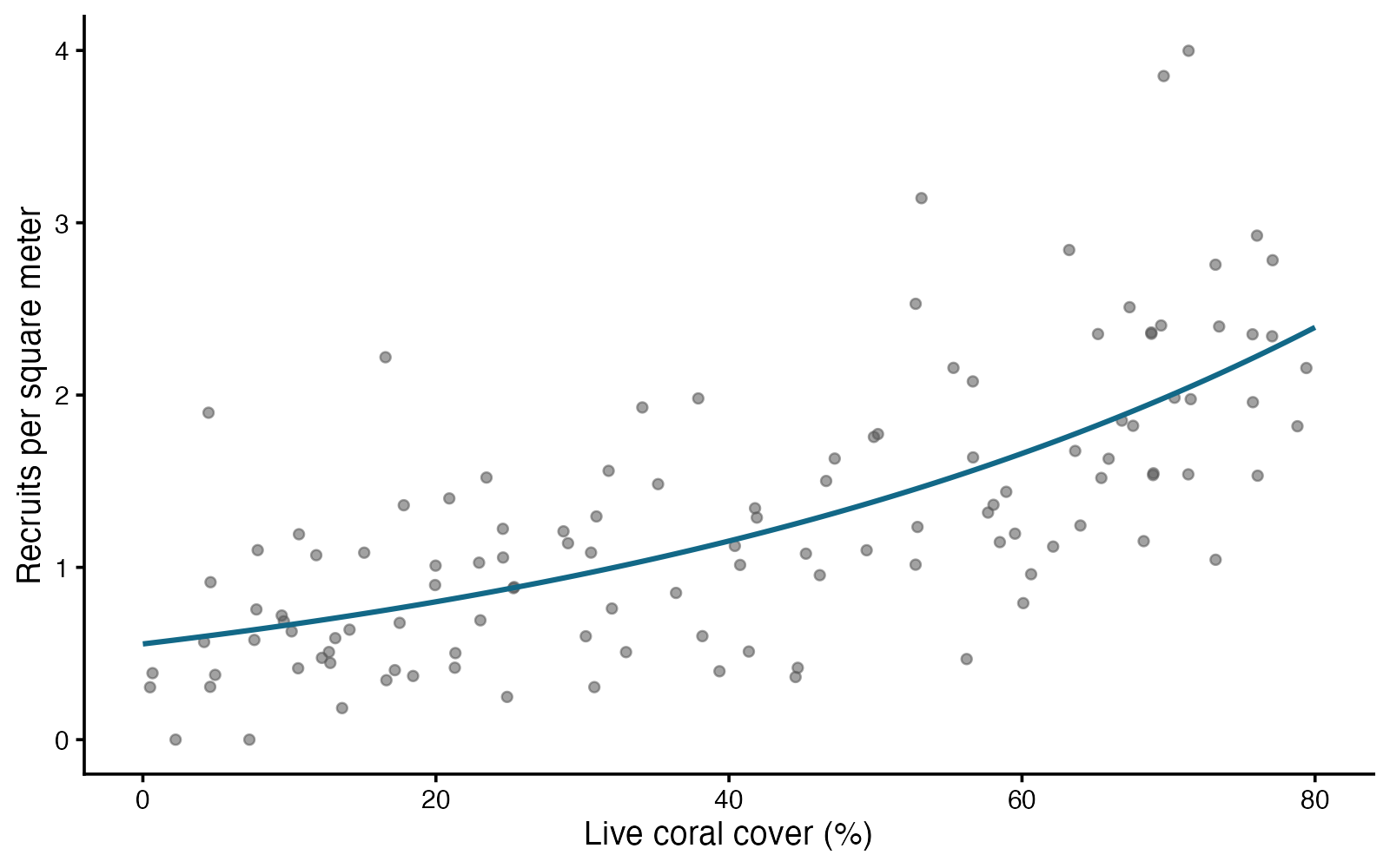
- Rate ratio per 10 cover points: 1.200
- 95% Wald CI: 1.162 to 1.240
- Likelihood-ratio p = 2.64e-30
- Pearson dispersion diagnostic: 1.111
A 10-percentage-point increase in coral cover multiplied modeled recruit density by 1.20 (95% Wald CI 1.16–1.24; p = 2.64e-30). Area is handled as exposure; the observational association is not a causal effect.
**Teaching point:** The exposure offset separates a biological density difference from simply looking over a larger area.
### Analysis code excerpt
```r
d <- read.csv("modules/poisson_glm/generated/data.csv")
fit <- glm(recruits ~ cover + offset(log(area)), data = d,
family = poisson)
p_value <- drop1(fit, test = "Chisq")["cover", "Pr(>Chi)"]
b <- coef(fit)["cover"]
se <- sqrt(vcov(fit)["cover", "cover"])
rate_ratio <- exp(10 * b)
ci <- exp(10 * (b + c(-1, 1) * 1.96 * se))
dispersion <- sum(residuals(fit, type = "pearson")^2) / df.residual(fit)
```
The full script supplies package loading and any additional preparation.
### Full printed R output
```text
Call:
glm(formula = recruits ~ cover + offset(log(area)), family = poisson,
data = d)
Coefficients:
Estimate Std. Error z value Pr(>|z|)
(Intercept) -0.587917 0.092543 -6.353 2.11e-10 ***
cover 0.018256 0.001649 11.071 < 2e-16 ***
---
Signif. codes: 0 ‘***’ 0.001 ‘**’ 0.01 ‘*’ 0.05 ‘.’ 0.1 ‘ ’ 1
(Dispersion parameter for poisson family taken to be 1)
Null deviance: 258.31 on 119 degrees of freedom
Residual deviance: 127.43 on 118 degrees of freedom
AIC: 541.72
Number of Fisher Scoring iterations: 4
```
### Recreate the observations
```r
out_dir <- "modules/poisson_glm/generated"
dir.create(out_dir, recursive = TRUE, showWarnings = FALSE)
set.seed(3111)
d <- data.frame(transect = 1:120, cover = runif(120, 0, 80),
area = runif(120, 2, 8))
d$recruits <- rpois(120, d$area * exp(-.5 + .016 * d$cover))
write.csv(d, file.path(out_dir, "data.csv"), row.names = FALSE)
```
Run the complete module from the course folder:
```sh
Rscript modules/poisson_glm/analysis.R modules/poisson_glm/generated
```
## Dataset 38: Quasi-Poisson regression
Bacterial colony counts with clumping
**Family:** Generalized linear models · **Rows:** 120 · **Seed:** 3113
[Saved CSV](modules/quasipoisson/generated/data.csv) · [Full runnable R script](modules/quasipoisson/analysis.R) · [Full-size plot](modules/quasipoisson/generated/plot.png)
**Generating truth:** High medium multiplies mean colony density by exp(0.5) ≈ 1.649; the equal-rate null is false. The true dispersion multiplier is 4, so Poisson uncertainty would be too small.
**Exact generating model:** Generate 60 low-medium and 60 high-medium independent plates, with volume Uniform(0.7,1.3) ml. Set mean count μ = volume × exp(2.4 + 0.5 × high). Generate clumps ~ Poisson(μ/3), then colonies ~ Poisson(3 × clumps). Marginal mean is μ and variance is 4μ.
**Scientific question:** Does mean colony density differ between media after accounting for plated volume?
**Null being tested / estimation target:** The high-medium coefficient is zero: mean colony rates are equal between media.
**Design and independent unit:** Independent plated samples vary in medium and plated volume.
### Columns
| Column | Meaning | Unit / type |
|---|---|---|
| medium | Low or High nutrient medium | none |
| volume_ml | Plated volume exposure | ml |
| colonies | Observed colony count after clumping | count |
### Analysis from the saved dataset
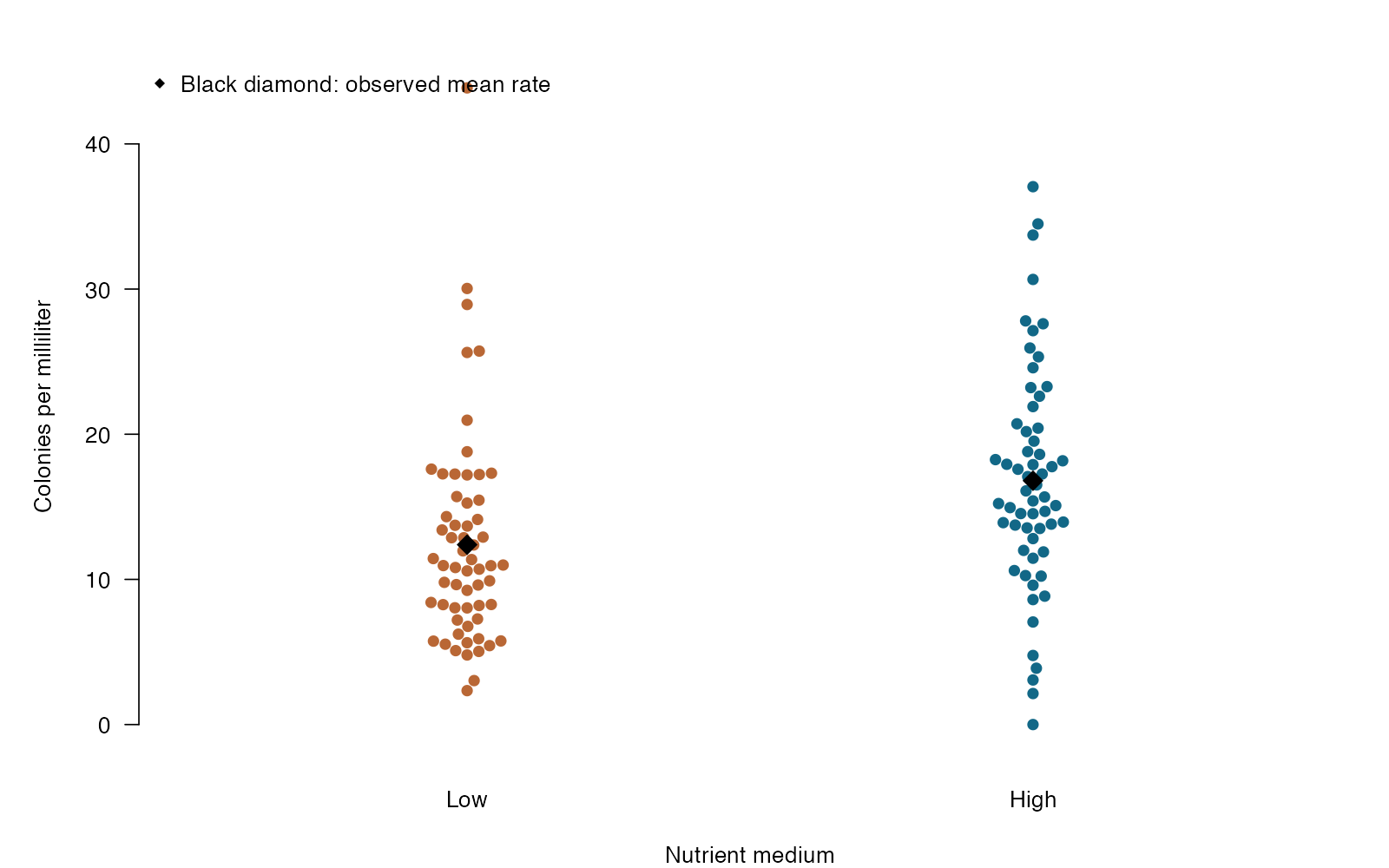
- High / low mean rate ratio: 1.351
- 95% t-based CI: 1.117 to 1.633
- Dispersion multiplier: 3.953
- Quasi-Poisson t-test p = 0.002166
High-nutrient medium had 1.35 times the modeled colony rate of low-nutrient medium (95% t-based CI 1.12–1.63; p = 0.00217). Estimated dispersion 3.95 adjusts uncertainty for extra-Poisson variation.
**Teaching point:** Quasi-Poisson retains the log-mean question while changing the uncertainty model; ordinary likelihood AIC is unavailable.
### Analysis code excerpt
```r
d <- read.csv("modules/quasipoisson/generated/data.csv")
d$medium <- factor(d$medium, levels = c("Low", "High"))
fit <- glm(colonies ~ medium + offset(log(volume_ml)),
data = d, family = quasipoisson)
b <- coef(fit)["mediumHigh"]
se <- sqrt(vcov(fit)["mediumHigh", "mediumHigh"])
critical <- qt(.975, df.residual(fit))
rate_ratio <- exp(b)
ci <- exp(b + c(-1, 1) * critical * se)
p_value <- summary(fit)$coefficients["mediumHigh", "Pr(>|t|)"]
```
The full script supplies package loading and any additional preparation.
### Full printed R output
```text
Call:
glm(formula = colonies ~ medium + offset(log(volume_ml)), family = quasipoisson,
data = d)
Coefficients:
Estimate Std. Error t value Pr(>|t|)
(Intercept) 2.52196 0.07284 34.622 < 2e-16 ***
mediumHigh 0.30075 0.09592 3.135 0.00217 **
---
Signif. codes: 0 ‘***’ 0.001 ‘**’ 0.01 ‘*’ 0.05 ‘.’ 0.1 ‘ ’ 1
(Dispersion parameter for quasipoisson family taken to be 3.953259)
Null deviance: 489.45 on 119 degrees of freedom
Residual deviance: 450.13 on 118 degrees of freedom
AIC: NA
Number of Fisher Scoring iterations: 4
```
### Recreate the observations
```r
out_dir <- "modules/quasipoisson/generated"
dir.create(out_dir, recursive = TRUE, showWarnings = FALSE)
set.seed(3113)
d <- data.frame(medium = rep(c("Low", "High"), each = 60),
volume_ml = runif(120, .7, 1.3))
mu <- d$volume_ml * exp(2.4 + .5 * (d$medium == "High"))
clumps <- rpois(120, mu / 3)
d$colonies <- rpois(120, 3 * clumps)
write.csv(d, file.path(out_dir, "data.csv"), row.names = FALSE)
```
Run the complete module from the course folder:
```sh
Rscript modules/quasipoisson/analysis.R modules/quasipoisson/generated
```
## Dataset 39: Negative binomial regression
Parasite abundance and fish body length
**Family:** Generalized linear models · **Rows:** 130 · **Seed:** 3112
[Saved CSV](modules/negbin_glm/generated/data.csv) · [Full runnable R script](modules/negbin_glm/analysis.R) · [Full-size plot](modules/negbin_glm/generated/plot.png)
**Generating truth:** The length coefficient is 0.085, so 5 cm multiplies expected parasite abundance by exp(0.425) ≈ 1.530. The slope-zero null is false; the Poisson variance assumption is intentionally violated.
**Exact generating model:** Generate 130 independent fish with length Uniform(18,42) cm. Parasite count follows a negative binomial with mean exp(-0.2 + 0.085 × length) and size/theta 2. Conditional variance is mean + mean²/2.
**Scientific question:** Does expected parasite burden change with fish length?
**Null being tested / estimation target:** The length coefficient is zero: expected parasite abundance does not change with length in this model.
**Design and independent unit:** Independent fish vary in body length; parasite burdens are highly variable.
### Columns
| Column | Meaning | Unit / type |
|---|---|---|
| fish | Unique independent fish identifier | none |
| length_cm | Fish body length | cm |
| parasites | Observed parasite burden | count |
### Analysis from the saved dataset
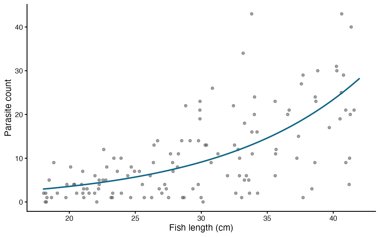
- Mean count ratio per 5 cm: 1.602
- 95% Wald CI: 1.458 to 1.761
- Wald p = 1.634e-22
- Estimated negative-binomial theta: 2.292
A 5-cm increase in fish length multiplied expected parasite count by 1.60 (95% Wald CI 1.46–1.76; Wald p = 1.63e-22). Negative binomial variation allows more spread than a Poisson model.
**Teaching point:** Overdispersion can be addressed with a parametric count model; it does not automatically require replacing the scientific question with a rank test.
### Analysis code excerpt
```r
d <- read.csv("modules/negbin_glm/generated/data.csv")
fit <- MASS::glm.nb(parasites ~ length_cm, data = d)
b <- coef(fit)["length_cm"]
se <- sqrt(vcov(fit)["length_cm", "length_cm"])
p_value <- summary(fit)$coefficients["length_cm", "Pr(>|z|)"]
rate_ratio <- exp(5 * b)
ci <- exp(5 * (b + c(-1, 1) * 1.96 * se))
```
The full script supplies package loading and any additional preparation.
### Full printed R output
```text
Call:
MASS::glm.nb(formula = parasites ~ length_cm, data = d, init.theta = 2.292042228,
link = log)
Coefficients:
Estimate Std. Error z value Pr(>|z|)
(Intercept) -0.617706 0.299553 -2.062 0.0392 *
length_cm 0.094281 0.009658 9.762 <2e-16 ***
---
Signif. codes: 0 ‘***’ 0.001 ‘**’ 0.01 ‘*’ 0.05 ‘.’ 0.1 ‘ ’ 1
(Dispersion parameter for Negative Binomial(2.292) family taken to be 1)
Null deviance: 234.38 on 129 degrees of freedom
Residual deviance: 140.90 on 128 degrees of freedom
AIC: 814.62
Number of Fisher Scoring iterations: 1
Theta: 2.292
Std. Err.: 0.374
2 x log-likelihood: -808.615
```
### Recreate the observations
```r
out_dir <- "modules/negbin_glm/generated"
dir.create(out_dir, recursive = TRUE, showWarnings = FALSE)
set.seed(3112)
d <- data.frame(fish = 1:130, length_cm = runif(130, 18, 42))
mu <- exp(-.2 + .085 * d$length_cm)
d$parasites <- rnbinom(130, mu = mu, size = 2)
write.csv(d, file.path(out_dir, "data.csv"), row.names = FALSE)
```
Run the complete module from the course folder:
```sh
Rscript modules/negbin_glm/analysis.R modules/negbin_glm/generated
```
## Dataset 40: Multinomial logistic regression
Fish use of three unordered feeding microhabitats
**Family:** Generalized linear models · **Rows:** 240 · **Seed:** 3114
[Saved CSV](modules/multinomial/generated/data.csv) · [Full runnable R script](modules/multinomial/analysis.R) · [Full-size plot](modules/multinomial/generated/plot.png)
**Generating truth:** The outcome distributions differ, so the joint no-food-effect null is false. Relative to Open, the food coefficients are log(0.30/0.50)-log(0.50/0.25) ≈ -1.204 for Shelter and log(0.20/0.50)-log(0.25/0.25) ≈ -0.916 for Surface.
**Exact generating model:** Generate 120 independent fish choices under Low food with Open/Shelter/Surface probabilities 0.25/0.50/0.25 and 120 under High food with probabilities 0.50/0.30/0.20. Choices are unordered, mutually exclusive, and independent.
**Scientific question:** Does food availability change the distribution of feeding microhabitat choices?
**Null being tested / estimation target:** All nonreference food coefficients are zero; microhabitat probabilities are the same under low and high food.
**Design and independent unit:** Independent fish encounter either low or high food availability.
### Columns
| Column | Meaning | Unit / type |
|---|---|---|
| food | Low or High food availability | none |
| choice | Open, Shelter, or Surface microhabitat | none |
### Analysis from the saved dataset
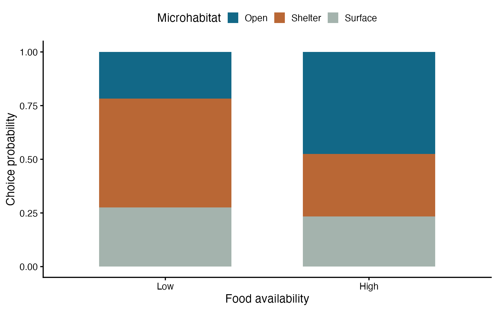
- Low-food probabilities: 0.217, 0.508, 0.275
- High-food probabilities: 0.475, 0.292, 0.233
- Likelihood ratio = 19.404; df = 2
- Joint p = 6.115e-05
Predicted probabilities for open/shelter/surface were 0.22/0.51/0.28 under low food and 0.48/0.29/0.23 under high food. The joint likelihood-ratio test gives chi-square(2) = 19.40, p = 6.11e-05; it tests the whole distribution of choices.
**Teaching point:** A categorical response with more than two levels requires a joint question across several coefficients.
### Analysis code excerpt
```r
d <- read.csv("modules/multinomial/generated/data.csv")
d$food <- factor(d$food, levels = c("Low", "High"))
d$choice <- factor(d$choice, levels = c("Open", "Shelter", "Surface"))
fit <- nnet::multinom(choice ~ food, data = d, trace = FALSE)
fit0 <- nnet::multinom(choice ~ 1, data = d, trace = FALSE)
LR <- 2 * as.numeric(logLik(fit) - logLik(fit0))
df <- attr(logLik(fit), "df") - attr(logLik(fit0), "df")
p_value <- pchisq(LR, df, lower.tail = FALSE)
```
The full script supplies package loading and any additional preparation.
### Full printed R output
```text
Call:
nnet::multinom(formula = choice ~ food, data = d, trace = FALSE)
Coefficients:
(Intercept) foodHigh
Shelter 0.8527665 -1.3404733
Surface 0.2384121 -0.9492706
Std. Errors:
(Intercept) foodHigh
Shelter 0.2342112 0.3177579
Surface 0.2622292 0.3493172
Residual Deviance: 499.8932
AIC: 507.8932
```
### Recreate the observations
```r
out_dir <- "modules/multinomial/generated"
dir.create(out_dir, recursive = TRUE, showWarnings = FALSE)
set.seed(3114)
d <- data.frame(food = rep(c("Low", "High"), each = 120))
d$choice <- c(sample(c("Open", "Shelter", "Surface"), 120, TRUE,
prob = c(.25, .50, .25)),
sample(c("Open", "Shelter", "Surface"), 120, TRUE,
prob = c(.50, .30, .20)))
write.csv(d, file.path(out_dir, "data.csv"), row.names = FALSE)
```
Run the complete module from the course folder:
```sh
Rscript modules/multinomial/analysis.R modules/multinomial/generated
```
## Dataset 41: Ordinal logistic regression
Coral bleaching severity along a temperature gradient
**Family:** Generalized linear models · **Rows:** 180 · **Seed:** 3115
[Saved CSV](modules/ordinal_logistic/generated/data.csv) · [Full runnable R script](modules/ordinal_logistic/analysis.R) · [Full-size plot](modules/ordinal_logistic/generated/plot.png)
**Generating truth:** The common temperature coefficient is 0.8, so each °C multiplies odds of higher versus lower severity by exp(0.8) ≈ 2.226 at every cumulative threshold. The zero-effect null is false and proportional odds holds by construction.
**Exact generating model:** Generate 180 independent fragments with temperature Uniform(26,32) °C. Latent severity is 0.8 × (temperature - 28) plus a standard logistic error. Cut at -1, 0.7, and 2.2 to obtain None, Mild, Moderate, Severe. Do not treat category spacing as numeric distance.
**Scientific question:** Does temperature shift bleaching severity toward higher ordered categories?
**Null being tested / estimation target:** The common temperature coefficient is zero; the modeled severity distribution does not change with temperature.
**Design and independent unit:** Independent coral fragments are assigned a four-level ordered bleaching score.
### Columns
| Column | Meaning | Unit / type |
|---|---|---|
| fragment | Unique independent coral fragment identifier | none |
| temperature | Experimental temperature | °C |
| severity | Ordered bleaching level: None < Mild < Moderate < Severe | none |
### Analysis from the saved dataset
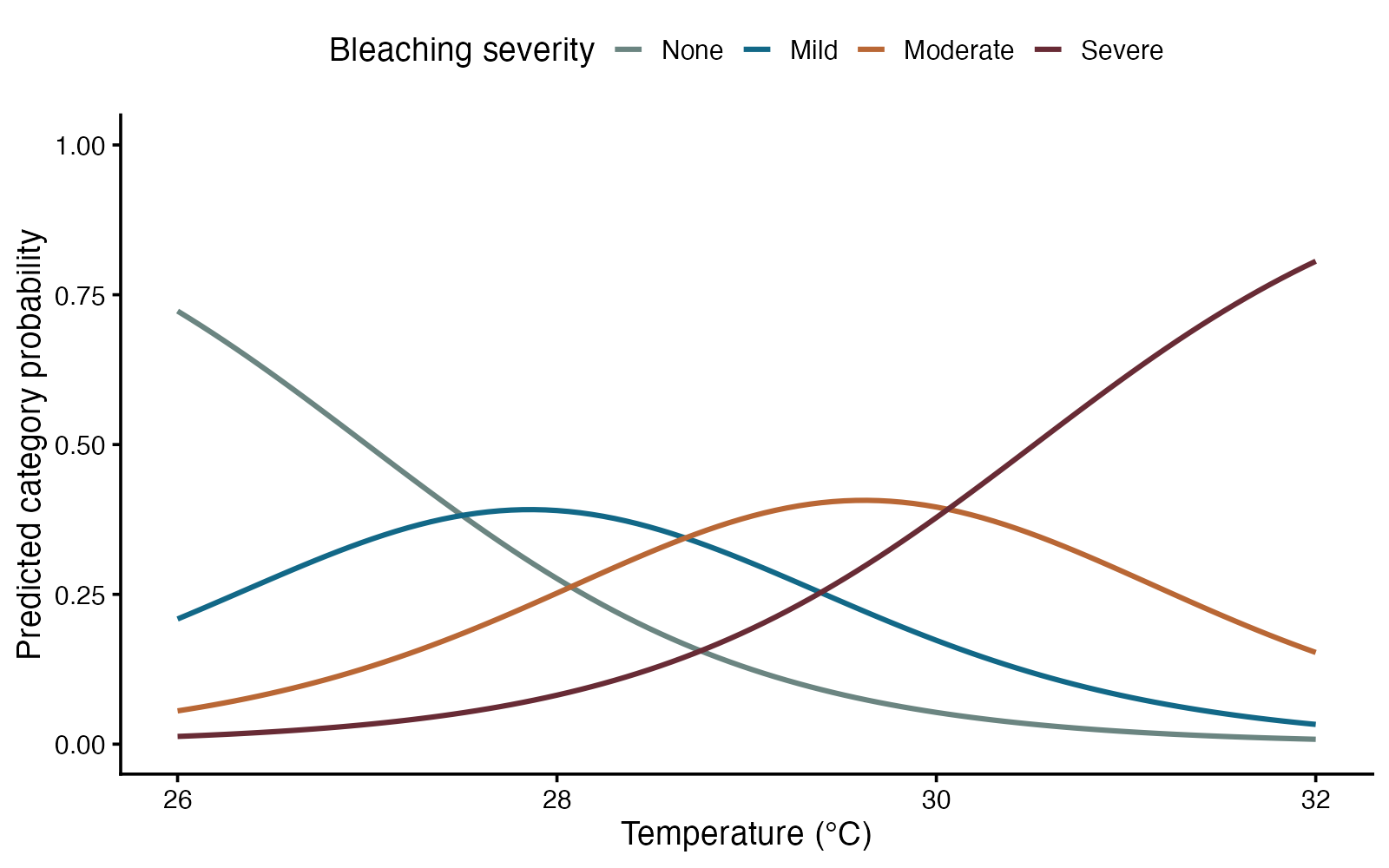
- Common odds ratio per 1°C: 2.613
- 95% Wald CI: 2.105 to 3.244
- Likelihood ratio = 97.836; df = 1
- p = 4.544e-23
Each 1°C increase multiplied the modeled odds of higher rather than lower bleaching severity by 2.61 (95% Wald CI 2.11–3.24; likelihood-ratio p = 4.54e-23), assuming the same temperature effect across thresholds.
**Teaching point:** Ordering carries information without assuming equal distances; the common effect across thresholds is the key model assumption.
### Analysis code excerpt
```r
d <- read.csv("modules/ordinal_logistic/generated/data.csv")
d$severity <- ordered(d$severity, levels = c("None", "Mild", "Moderate", "Severe"))
fit <- ordinal::clm(severity ~ temperature, data = d, link = "logit")
fit0 <- ordinal::clm(severity ~ 1, data = d, link = "logit")
LR <- 2 * as.numeric(logLik(fit) - logLik(fit0))
p_value <- pchisq(LR, df = 1, lower.tail = FALSE)
b <- fit$beta["temperature"]
se <- sqrt(vcov(fit)["temperature", "temperature"])
odds_ratio <- exp(b)
ci <- exp(b + c(-1, 1) * 1.96 * se)
```
The full script supplies package loading and any additional preparation.
### Full printed R output
```text
formula: severity ~ temperature
data: d
link threshold nobs logLik AIC niter max.grad cond.H
logit flexible 180 -200.34 408.69 5(0) 2.85e-11 1.3e+06
Coefficients:
Estimate Std. Error z value Pr(>|z|)
temperature 0.9606 0.1103 8.71 <2e-16 ***
---
Signif. codes: 0 ‘***’ 0.001 ‘**’ 0.01 ‘*’ 0.05 ‘.’ 0.1 ‘ ’ 1
Threshold coefficients:
Estimate Std. Error z value
None|Mild 25.935 3.098 8.373
Mild|Moderate 27.589 3.178 8.682
Moderate|Severe 29.316 3.273 8.957
```
### Recreate the observations
```r
out_dir <- "modules/ordinal_logistic/generated"
dir.create(out_dir, recursive = TRUE, showWarnings = FALSE)
set.seed(3115)
d <- data.frame(fragment = 1:180, temperature = runif(180, 26, 32))
latent <- .8 * (d$temperature - 28) + rlogis(180)
d$severity <- cut(latent, c(-Inf, -1, .7, 2.2, Inf),
labels = c("None", "Mild", "Moderate", "Severe"))
write.csv(d, file.path(out_dir, "data.csv"), row.names = FALSE)
```
Run the complete module from the course folder:
```sh
Rscript modules/ordinal_logistic/analysis.R modules/ordinal_logistic/generated
```
## Dataset 42: Linear mixed model
Evolutionary biologists follow larval growth under two diets.
**Family:** Repeated and clustered data · **Rows:** 144 · **Seed:** 2106
[Saved CSV](modules/linear_mixed/generated/data.csv) · [Full runnable R script](modules/linear_mixed/analysis.R) · [Full-size plot](modules/linear_mixed/generated/plot.png)
**Generating truth:** The control slope is 2 mg/week; enrichment adds 0.9 mg/week. The diet-by-week null is false. Simulated random-intercept and slope SDs are 2.3 mg and 0.7 mg/week.
**Exact generating model:** 36 larvae (18 per diet) are measured at weeks 0–3. Mass = 12 + 2 × week + 0.8 if enriched + 0.9 × week if enriched + a larval Normal(0, 2.3²) intercept + a larval Normal(0, 0.7²) slope × week + independent Normal(0, 1.1²) error. Simulated intercepts and slopes are independent. Repeated values share both effects; no rounding.
**Scientific question:** Does diet change the mean growth slope?
**Null being tested / estimation target:** The population growth-slope difference between diets is zero.
**Design and independent unit:** 36 larvae measured at weeks 0–3; diet assigned to larvae.
### Columns
| Column | Meaning | Unit / type |
|---|---|---|
| week | Time since baseline | week |
| larva | Repeated biological individual | ID |
| treatment | Control or enriched diet | category |
| mass | Larval mass | mg |
### Analysis from the saved dataset
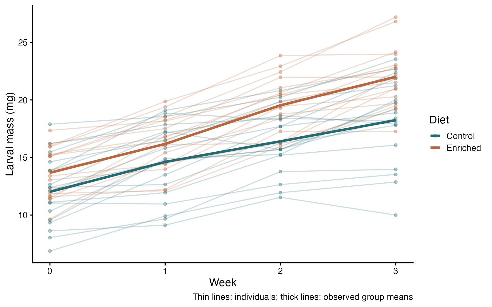
- Growth-slope difference = 0.79 mg/week
- Approximate 95% Wald CI 0.31 to 1.27
- Satterthwaite df = 34.0; t = 3.20; p = 0.002966
- 36 larvae; 144 rows; singular fit: FALSE
Enrichment increased the fitted growth slope by 0.79 mg/week (approximate 95% Wald CI 0.31 to 1.27; Satterthwaite t with 34.0 df, p = 0.002966). Individual intercepts and slopes model repeated larvae; 144 rows do not represent 144 independent animals.
**Teaching point:** Random intercepts describe starting differences; random slopes describe trajectory differences.
### Analysis code excerpt
```r
d <- read.csv("modules/linear_mixed/generated/data.csv")
fit <- lmerTest::lmer(mass ~ treatment * week + (week | larva), data = d)
summary(fit, ddf = "Satterthwaite")
trend_ci <- confint(fit, parm = "treatmentEnriched:week", method = "Wald")
```
The full script supplies package loading and any additional preparation.
### Full printed R output
```text
Linear mixed model fit by REML. t-tests use Satterthwaite's method [
lmerModLmerTest]
Formula: mass ~ treatment * week + (week | larva)
Data: d
REML criterion at convergence: 570
Scaled residuals:
Min 1Q Median 3Q Max
-1.64582 -0.56247 0.05774 0.54128 1.60492
Random effects:
Groups Name Variance Std.Dev. Corr
larva (Intercept) 5.7165 2.3909
week 0.3129 0.5594 -0.01
Residual 1.1701 1.0817
Number of obs: 144, groups: larva, 36
Fixed effects:
Estimate Std. Error df t value Pr(>|t|)
(Intercept) 12.2501 0.6026 33.9995 20.330 < 2e-16 ***
treatmentEnriched 1.3465 0.8522 33.9995 1.580 0.12335
week 2.0463 0.1743 34.0002 11.740 1.65e-13 ***
treatmentEnriched:week 0.7891 0.2465 34.0002 3.201 0.00297 **
---
Signif. codes: 0 ‘***’ 0.001 ‘**’ 0.01 ‘*’ 0.05 ‘.’ 0.1 ‘ ’ 1
Correlation of Fixed Effects:
(Intr) trtmnE week
trtmntEnrch -0.707
week -0.193 0.137
trtmntEnrc: 0.137 -0.193 -0.707
```
### Recreate the observations
```r
output_dir <- "modules/linear_mixed/generated"
dir.create(output_dir, recursive = TRUE, showWarnings = FALSE)
set.seed(2106)
d <- expand.grid(week = 0:3, larva = 1:36)
d$treatment <- rep(rep(c("Control", "Enriched"), each = 18), each = 4)
intercepts <- rnorm(36, 0, 2.3); slopes <- rnorm(36, 0, .7)
d$mass <- 12 + 2 * d$week + .8 * (d$treatment == "Enriched") +
.9 * d$week * (d$treatment == "Enriched") + intercepts[d$larva] +
slopes[d$larva] * d$week + rnorm(nrow(d), 0, 1.1)
write.csv(d, file.path(output_dir, "data.csv"), row.names = FALSE)
```
Run the complete module from the course folder:
```sh
Rscript modules/linear_mixed/analysis.R modules/linear_mixed/generated
```
## Dataset 43: Binary mixed model
Immunologists record repeated infection outcomes in vaccinated and control hosts.
**Family:** Repeated and clustered data · **Rows:** 288 · **Seed:** 2107
[Saved CSV](modules/binary_glmm/generated/data.csv) · [Full runnable R script](modules/binary_glmm/analysis.R) · [Full-size plot](modules/binary_glmm/generated/plot.png)
**Generating truth:** The conditional vaccine odds ratio is exp(−1) ≈ 0.368; the week odds ratio is exp(0.25) ≈ 1.284. The vaccine null is false. These are conditional effects, not population-average odds ratios.
**Exact generating model:** 72 hosts (36 per group) are scored at weeks 0–3. Host intercepts are Normal(0, 0.8²). The infection log odds equal −0.4 + 0.25 × week − 1.0 if vaccinated + host intercept. Independent Bernoulli outcomes are sampled conditional on those probabilities. Host intercepts create dependence across visits; latent probabilities are removed from the saved student dataset.
**Scientific question:** Does vaccination affect infection odds while accounting for repeated hosts?
**Null being tested / estimation target:** The vaccination coefficient is zero: its conditional odds ratio is one.
**Design and independent unit:** 72 hosts with four weekly binary responses.
### Columns
| Column | Meaning | Unit / type |
|---|---|---|
| week | Scheduled visit relative to baseline | week |
| host | Repeated host identifier | ID |
| treatment | Control or vaccine assignment | category |
| infected | Infection outcome: 1 infected, 0 not infected | binary |
### Analysis from the saved dataset
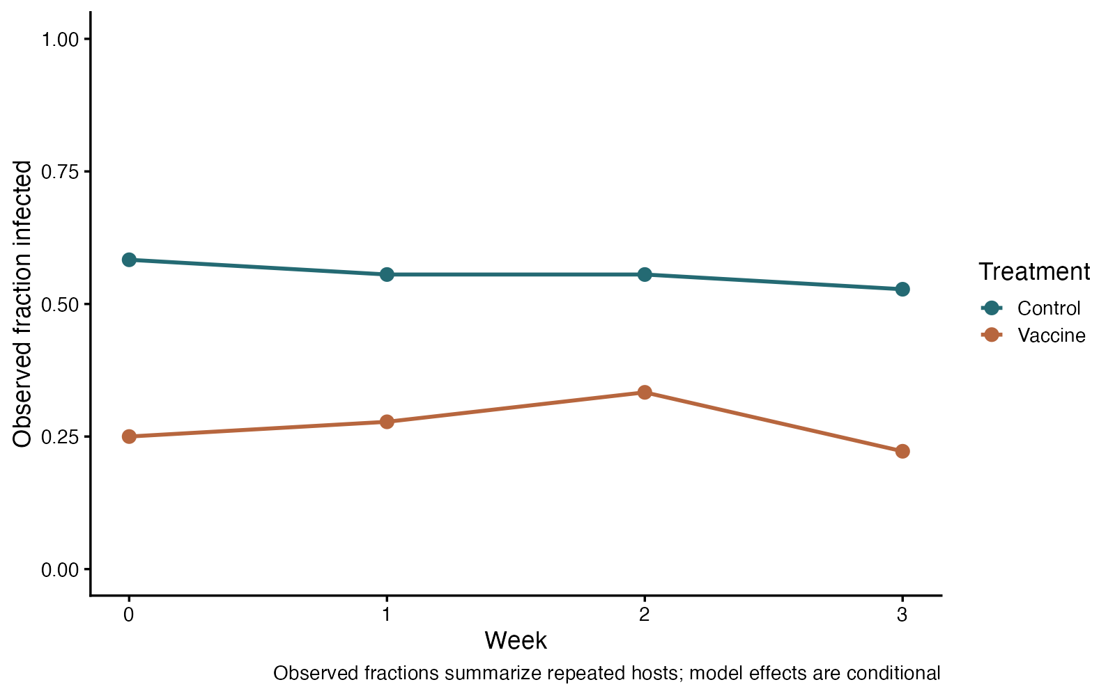
- Conditional vaccine odds ratio = 0.24
- Approximate 95% CI 0.12 to 0.48
- Wald z = -3.99; p = 6.63e-05
- 72 independent hosts; four repeated observations each
At the same week and host random effect, vaccination multiplied infection odds by 0.24 (approximate 95% Wald CI 0.12 to 0.48; p = 6.63e-05). This is a conditional odds ratio, not a probability ratio or the population-average odds ratio estimated by a GEE.
**Teaching point:** Repeated binary outcomes need both a response distribution and a dependence model.
### Analysis code excerpt
```r
d <- read.csv("modules/binary_glmm/generated/data.csv")
fit <- lme4::glmer(infected ~ treatment + week + (1 | host),
family = binomial, data = d,
control = lme4::glmerControl(optimizer = "bobyqa"))
summary(fit)
log_or_ci <- confint(fit, parm = "treatmentVaccine", method = "Wald")
```
The full script supplies package loading and any additional preparation.
### Full printed R output
```text
Generalized linear mixed model fit by maximum likelihood (Laplace
Approximation) [glmerMod]
Family: binomial ( logit )
Formula: infected ~ treatment + week + (1 | host)
Data: d
Control: lme4::glmerControl(optimizer = "bobyqa")
AIC BIC logLik -2*log(L) df.resid
366.0 380.7 -179.0 358.0 284
Scaled residuals:
Min 1Q Median 3Q Max
-1.4049 -0.6888 -0.4268 0.7494 1.8362
Random effects:
Groups Name Variance Std.Dev.
host (Intercept) 0.8177 0.9043
Number of obs: 288, groups: host, 72
Fixed effects:
Estimate Std. Error z value Pr(>|z|)
(Intercept) 0.34030 0.29953 1.136 0.256
treatmentVaccine -1.42502 0.35722 -3.989 6.63e-05 ***
week -0.05141 0.12047 -0.427 0.670
---
Signif. codes: 0 ‘***’ 0.001 ‘**’ 0.01 ‘*’ 0.05 ‘.’ 0.1 ‘ ’ 1
Correlation of Fixed Effects:
(Intr) trtmnV
tretmntVccn -0.550
week -0.607 0.016
```
### Recreate the observations
```r
output_dir <- "modules/binary_glmm/generated"
dir.create(output_dir, recursive = TRUE, showWarnings = FALSE)
set.seed(2107)
d <- expand.grid(week = 0:3, host = 1:72)
d$treatment <- rep(rep(c("Control", "Vaccine"), each = 36), each = 4)
individual <- rnorm(72, 0, .8)
d$probability <- plogis(-.4 + .25 * d$week -
1.0 * (d$treatment == "Vaccine") + individual[d$host])
d$infected <- rbinom(nrow(d), 1, d$probability)
d$probability <- NULL
write.csv(d, file.path(output_dir, "data.csv"), row.names = FALSE)
```
Run the complete module from the course folder:
```sh
Rscript modules/binary_glmm/analysis.R modules/binary_glmm/generated
```
## Dataset 44: Count mixed model: Poisson and negative binomial
Pollinator visits are repeatedly counted on plants in two habitats.
**Family:** Repeated and clustered data · **Rows:** 192 · **Seed:** 2114
[Saved CSV](modules/count_glmm/generated/data.csv) · [Full runnable R script](modules/count_glmm/analysis.R) · [Full-size plot](modules/count_glmm/generated/plot.png)
**Generating truth:** The conditional sheltered/open rate ratio is exp(0.55) ≈ 1.733; the habitat null is false. The generating distribution has extra variation beyond Poisson even after conditioning on the plant intercept.
**Exact generating model:** 48 plants (24 per habitat) are observed on days 1–4. Observation duration is sampled uniformly from the integers 20–60 minutes. Plant intercepts are Normal(0, 0.45²). Log rate = −2 + 0.55 if sheltered + 0.06 × day + plant intercept. Counts are negative binomial with mean = minutes × rate and size = 5; conditional variance is mean + mean²/5. Repeated plants share the intercept.
**Scientific question:** Does habitat change visit rate while accounting for repeated plants?
**Null being tested / estimation target:** The habitat coefficient is zero: its conditional visit-rate ratio is one.
**Design and independent unit:** 48 plants observed on four days with unequal observation durations.
### Columns
| Column | Meaning | Unit / type |
|---|---|---|
| day | Observation day | day |
| plant | Repeated plant identifier | ID |
| habitat | Open or sheltered habitat | category |
| minutes | Observation exposure | minute |
| visits | Number of pollinator visits | count |
### Analysis from the saved dataset
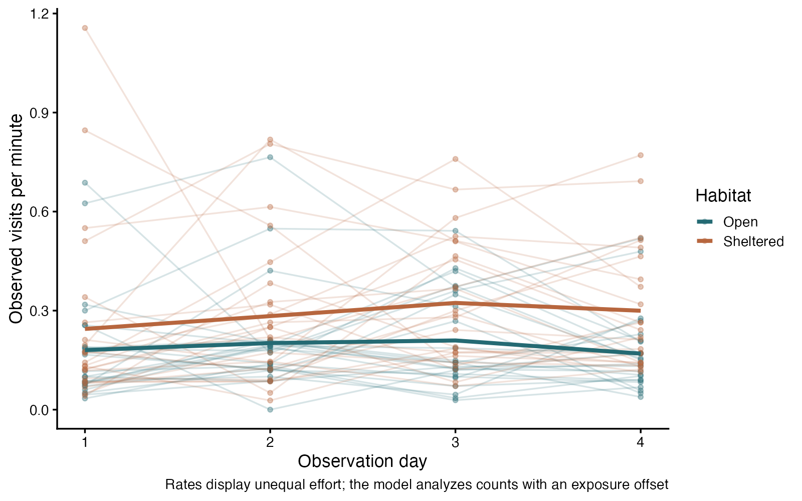
- Conditional sheltered/open rate ratio = 1.50
- Approximate 95% CI 1.11 to 2.02
- Wald z = 2.62; p = 0.008759
- Poisson AIC 1281.6; negative-binomial AIC 1165.5
In the negative-binomial mixed model, sheltered plants had 1.50 times the visit rate of open plants at the same day and random effect (approximate 95% Wald CI 1.11 to 2.02; p = 0.008759). Minutes are an exposure offset; plant intercepts model repeated observations. Extra conditional variation motivates checking the negative-binomial variant, not automatically selecting it from a single cutoff.
**Teaching point:** Offsets retain count information while accounting for exposure; negative binomial and random effects address different variation sources.
### Analysis code excerpt
```r
d <- read.csv("modules/count_glmm/generated/data.csv")
poisson_fit <- lme4::glmer(visits ~ habitat + day +
offset(log(minutes)) + (1 | plant), family = poisson, data = d,
control = lme4::glmerControl(optimizer = "bobyqa"))
fit <- lme4::glmer.nb(visits ~ habitat + day +
offset(log(minutes)) + (1 | plant), data = d,
control = lme4::glmerControl(optimizer = "bobyqa"))
summary(fit)
log_ratio_ci <- confint(fit, parm = "habitatSheltered", method = "Wald")
```
The full script supplies package loading and any additional preparation.
### Full printed R output
```text
Generalized linear mixed model fit by maximum likelihood (Laplace
Approximation) [glmerMod]
Family: Negative Binomial(5.8365) ( log )
Formula: visits ~ habitat + day + offset(log(minutes)) + (1 | plant)
Data: d
Control: lme4::glmerControl(optimizer = "bobyqa")
AIC BIC logLik -2*log(L) df.resid
1165.5 1181.8 -577.8 1155.5 187
Scaled residuals:
Min 1Q Median 3Q Max
-1.6584 -0.6798 -0.1409 0.4246 3.2452
Random effects:
Groups Name Variance Std.Dev.
plant (Intercept) 0.2057 0.4536
Number of obs: 192, groups: plant, 48
Fixed effects:
Estimate Std. Error z value Pr(>|z|)
(Intercept) -1.90884 0.14304 -13.345 < 2e-16 ***
habitatSheltered 0.40249 0.15355 2.621 0.00876 **
day 0.05234 0.03605 1.452 0.14658
---
Signif. codes: 0 ‘***’ 0.001 ‘**’ 0.01 ‘*’ 0.05 ‘.’ 0.1 ‘ ’ 1
Correlation of Fixed Effects:
(Intr) hbttSh
habttShltrd -0.547
day -0.638 -0.005
Generalized linear mixed model fit by maximum likelihood (Laplace
Approximation) [glmerMod]
Family: poisson ( log )
Formula: visits ~ habitat + day + offset(log(minutes)) + (1 | plant)
Data: d
Control: lme4::glmerControl(optimizer = "bobyqa")
AIC BIC logLik -2*log(L) df.resid
1281.6 1294.7 -636.8 1273.6 188
Scaled residuals:
Min 1Q Median 3Q Max
-3.0928 -0.9462 -0.1606 0.6940 5.4685
Random effects:
Groups Name Variance Std.Dev.
plant (Intercept) 0.2447 0.4947
Number of obs: 192, groups: plant, 48
Fixed effects:
Estimate Std. Error z value Pr(>|z|)
(Intercept) -1.90548 0.12177 -15.649 <2e-16 ***
habitatSheltered 0.40022 0.15209 2.631 0.0085 **
day 0.04840 0.02086 2.321 0.0203 *
---
Signif. codes: 0 ‘***’ 0.001 ‘**’ 0.01 ‘*’ 0.05 ‘.’ 0.1 ‘ ’ 1
Correlation of Fixed Effects:
(Intr) hbttSh
habttShltrd -0.644
day -0.447 0.011
```
### Recreate the observations
```r
output_dir <- "modules/count_glmm/generated"
dir.create(output_dir, recursive = TRUE, showWarnings = FALSE)
set.seed(2114)
d <- expand.grid(day = 1:4, plant = 1:48)
d$habitat <- rep(rep(c("Open", "Sheltered"), each = 24), each = 4)
d$minutes <- sample(20:60, nrow(d), replace = TRUE)
individual <- rnorm(48, 0, .45)
rate <- exp(-2.0 + .55 * (d$habitat == "Sheltered") +
.06 * d$day + individual[d$plant])
d$visits <- rnbinom(nrow(d), mu = d$minutes * rate, size = 5)
write.csv(d, file.path(output_dir, "data.csv"), row.names = FALSE)
```
Run the complete module from the course folder:
```sh
Rscript modules/count_glmm/analysis.R modules/count_glmm/generated
```
## Dataset 45: Ordinal mixed model
Fish behavior is scored repeatedly using ordered stress categories.
**Family:** Repeated and clustered data · **Rows:** 210 · **Seed:** 2109
[Saved CSV](modules/ordinal_mixed/generated/data.csv) · [Full runnable R script](modules/ordinal_mixed/analysis.R) · [Full-size plot](modules/ordinal_mixed/generated/plot.png)
**Generating truth:** The conditional common odds ratio for a higher score under stress is exp(0.8) ≈ 2.226. The treatment null is false. The simulated thresholds obey proportional odds.
**Exact generating model:** 70 fish (35 per treatment) are scored at visits 1–3. Fish intercepts are Normal(0, 0.8²). Latent severity = 0.8 if stressed + 0.15 × visit + fish intercept + standard logistic error. Thresholds −0.8, 0.3 and 1.3 produce None, Mild, Moderate and High. The latent score is not saved; repeated scores share the fish intercept.
**Scientific question:** Does treatment shift repeated scores toward higher categories?
**Null being tested / estimation target:** The treatment coefficient is zero: its conditional cumulative odds ratio is one.
**Design and independent unit:** 70 fish measured at three visits; treatment assigned between fish.
### Columns
| Column | Meaning | Unit / type |
|---|---|---|
| visit | Scheduled repeated assessment | visit |
| fish | Repeated fish identifier | ID |
| treatment | Control or stress assignment | category |
| score | Ordered behavior severity | ordered category |
### Analysis from the saved dataset
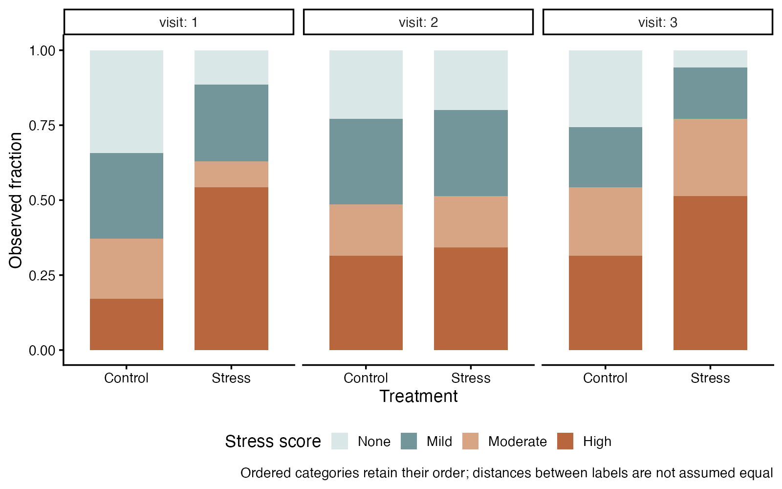
- Conditional higher-score odds ratio = 2.51
- Approximate 95% CI 1.31 to 4.82
- Wald z = 2.78; p = 0.005491
- 70 fish; three repeated ordinal scores each
At the same visit and fish random effect, stress treatment multiplied the odds of being above any score threshold by 2.51 (approximate 95% Wald CI 1.31 to 4.82; p = 0.005491). The proportional-odds model uses a common effect across thresholds; category labels are ordered, not equally spaced measurements.
**Teaching point:** Use ordered category probabilities; arbitrary numerical category spacings are unnecessary.
### Analysis code excerpt
```r
d <- read.csv("modules/ordinal_mixed/generated/data.csv")
fit <- ordinal::clmm(score ~ treatment + visit + (1 | fish),
data = d, link = "logit", Hess = TRUE)
summary(fit)
b <- coef(summary(fit))["treatmentStress", ]
log_or_ci <- b[1] + c(-1, 1) * qnorm(.975) * b[2]
```
The full script supplies package loading and any additional preparation.
### Full printed R output
```text
Cumulative Link Mixed Model fitted with the Laplace approximation
formula: score ~ treatment + visit + (1 | fish)
data: d
link threshold nobs logLik AIC niter max.grad cond.H
logit flexible 210 -274.11 560.22 240(723) 5.81e-05 1.0e+02
Random effects:
Groups Name Variance Std.Dev.
fish (Intercept) 0.6701 0.8186
Number of groups: fish 70
Coefficients:
Estimate Std. Error z value Pr(>|z|)
treatmentStress 0.9221 0.3321 2.777 0.00549 **
visit 0.2399 0.1608 1.492 0.13578
---
Signif. codes: 0 ‘***’ 0.001 ‘**’ 0.01 ‘*’ 0.05 ‘.’ 0.1 ‘ ’ 1
Threshold coefficients:
Estimate Std. Error z value
None|Mild -0.6966 0.4029 -1.729
Mild|Moderate 0.6908 0.4025 1.716
Moderate|High 1.5974 0.4207 3.797
```
### Recreate the observations
```r
output_dir <- "modules/ordinal_mixed/generated"
dir.create(output_dir, recursive = TRUE, showWarnings = FALSE)
set.seed(2109)
d <- expand.grid(visit = 1:3, fish = 1:70)
d$treatment <- rep(rep(c("Control", "Stress"), each = 35), each = 3)
individual <- rnorm(70, 0, .8)
latent <- .8 * (d$treatment == "Stress") + .15 * d$visit +
individual[d$fish] + rlogis(nrow(d))
d$score <- cut(latent, c(-Inf, -.8, .3, 1.3, Inf),
labels = c("None", "Mild", "Moderate", "High"))
write.csv(d, file.path(output_dir, "data.csv"), row.names = FALSE)
```
Run the complete module from the course folder:
```sh
Rscript modules/ordinal_mixed/analysis.R modules/ordinal_mixed/generated
```
## Dataset 46: Binary generalized estimating equations
Repeated infection screening after vaccination
**Family:** Dependent observations · **Rows:** 320 · **Seed:** 3116
[Saved CSV](modules/binary_gee/generated/data.csv) · [Full runnable R script](modules/binary_gee/analysis.R) · [Full-size plot](modules/binary_gee/generated/plot.png)
**Generating truth:** The true population-average vaccination coefficient is -0.9 and odds ratio exp(-0.9) ≈ 0.407, adjusted for week. The no-group-effect null is false. The true marginal week coefficient is 0.35. A working exchangeable correlation is an approximation, while the marginal mean model is exact.
**Exact generating model:** Generate 80 independent animals, 40 per vaccination group, measured at weeks 0,1,2,3. Set the marginal infection probability to plogis(-0.6 + 0.35 × week - 0.9 × vaccinated). For each row, z = sqrt(0.3) × shared animal Normal(0,1) + sqrt(0.7) × independent Normal(0,1). Because each z is standard normal, pnorm(z) is marginally uniform. Infection is 1 when pnorm(z) is below the specified probability. The shared component creates dependence while preserving the exact marginal probabilities.
**Scientific question:** Does population-average infection probability differ by vaccination after accounting for week?
**Null being tested / estimation target:** The population-average vaccination coefficient is zero, adjusting for week.
**Design and independent unit:** 80 independent animals are screened at four scheduled visits.
### Columns
| Column | Meaning | Unit / type |
|---|---|---|
| animal | Independent animal and clustering identifier | none |
| week | Scheduled visit time | weeks |
| vaccine | Control or Vaccinated group | none |
| infected | 1 = infection detected; 0 = not detected | binary |
### Analysis from the saved dataset
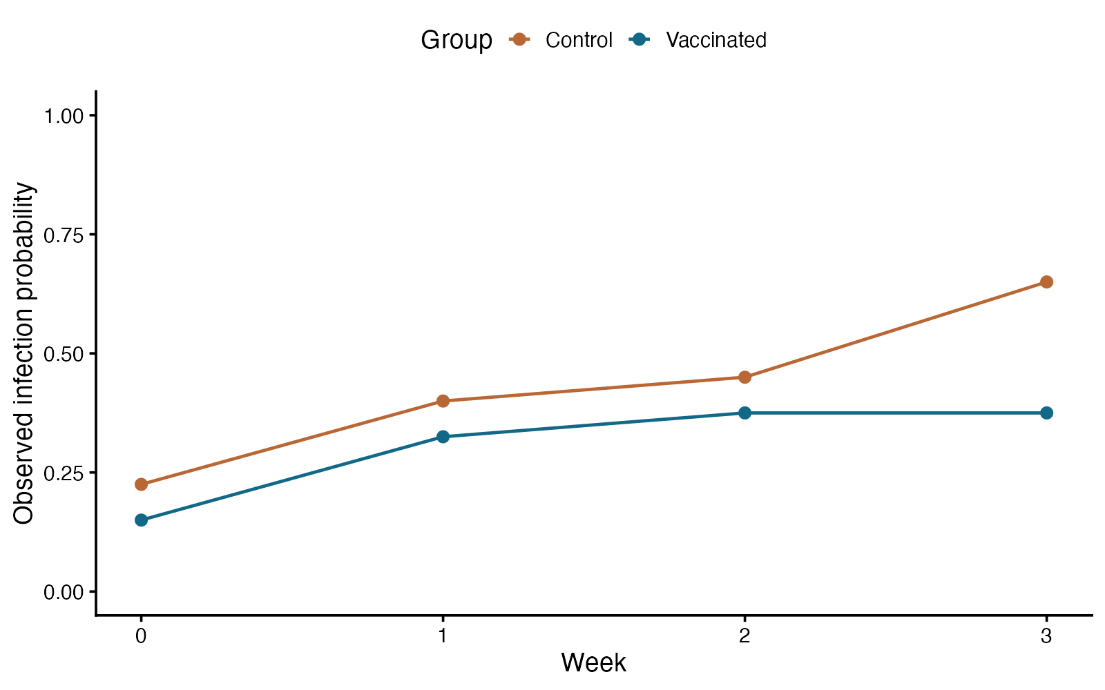
- Independent animals: 80; observations: 320
- Marginal vaccination odds ratio: 0.555
- 95% robust CI: 0.294 to 1.046
- Robust Wald p = 0.06864
- Working correlation estimate: 0.265
The estimated population-average infection odds ratio for vaccination was 0.55 (95% robust CI 0.29–1.05; Wald p = 0.0686), adjusted for week. The model treats 80 animals, rather than 320 rows, as independent units.
**Teaching point:** Choose between a population-average question and an individual-conditional question; repeated rows are not independent animals.
### Analysis code excerpt
```r
d <- read.csv("modules/binary_gee/generated/data.csv")
d$vaccine <- factor(d$vaccine, levels = c("Control", "Vaccinated"))
d <- d[order(d$animal, d$week), ]
fit <- geepack::geeglm(infected ~ vaccine + week, id = animal,
data = d, family = binomial, corstr = "exchangeable")
b <- coef(fit)["vaccineVaccinated"]
se <- sqrt(vcov(fit)["vaccineVaccinated", "vaccineVaccinated"])
odds_ratio <- exp(b)
ci <- exp(b + c(-1, 1) * 1.96 * se)
p_value <- 2 * pnorm(abs(b / se), lower.tail = FALSE)
```
The full script supplies package loading and any additional preparation.
### Full printed R output
```text
Call:
geepack::geeglm(formula = infected ~ vaccine + week, family = binomial,
data = d, id = animal, corstr = "exchangeable")
Coefficients:
Estimate Std.err Wald Pr(>|W|)
(Intercept) -0.98785 0.25570 14.926 0.000112 ***
vaccineVaccinated -0.58896 0.32346 3.315 0.068637 .
week 0.46535 0.08719 28.486 9.44e-08 ***
---
Signif. codes: 0 ‘***’ 0.001 ‘**’ 0.01 ‘*’ 0.05 ‘.’ 0.1 ‘ ’ 1
Correlation structure = exchangeable
Estimated Scale Parameters:
Estimate Std.err
(Intercept) 1 0.08157
Link = identity
Estimated Correlation Parameters:
Estimate Std.err
alpha 0.2655 0.0796
Number of clusters: 80 Maximum cluster size: 4
```
### Recreate the observations
```r
out_dir <- "modules/binary_gee/generated"
dir.create(out_dir, recursive = TRUE, showWarnings = FALSE)
set.seed(3116)
shared <- rep(rnorm(80), each = 4)
d <- data.frame(animal = rep(1:80, each = 4),
week = rep(0:3, 80), vaccine = rep(rep(c("Control", "Vaccinated"), each = 40), each = 4))
z <- sqrt(.3) * shared + sqrt(.7) * rnorm(320)
p <- plogis(-.6 + .35 * d$week - .9 * (d$vaccine == "Vaccinated"))
d$infected <- as.integer(pnorm(z) < p)
write.csv(d, file.path(out_dir, "data.csv"), row.names = FALSE)
```
Run the complete module from the course folder:
```sh
Rscript modules/binary_gee/analysis.R modules/binary_gee/generated
```
## Dataset 47: Kaplan–Meier survival estimation
Ecologists follow seedling survival until death or final observation.
**Family:** Time to event · **Rows:** 120 · **Seed:** 2110
[Saved CSV](modules/kaplan_meier/generated/data.csv) · [Full runnable R script](modules/kaplan_meier/analysis.R) · [Full-size plot](modules/kaplan_meier/generated/plot.png)
**Generating truth:** The population survival function is exp(−0.018 × days); true day-40 survival is exp(−0.72) ≈ 0.487. This is an estimation target, not a null hypothesis.
**Exact generating model:** 120 independent event times are drawn from an exponential distribution with death rate 0.018/day. Each independent final follow-up time is Uniform(35, 100) days. Observed days = minimum(event time, follow-up); event = 1 when the event occurs by follow-up and 0 otherwise. Times remain unrounded. Censoring is independent by construction.
**Scientific question:** What fraction of seedlings remain alive at day 40?
**Null being tested / estimation target:** No null hypothesis: the target is the survival probability over time.
**Design and independent unit:** 120 independent seedlings; follow-up ends at different times.
### Columns
| Column | Meaning | Unit / type |
|---|---|---|
| seedling | Independent seedling identifier | ID |
| days | Observed event or censoring time | day |
| event | 1 death; 0 right-censored | binary |
### Analysis from the saved dataset
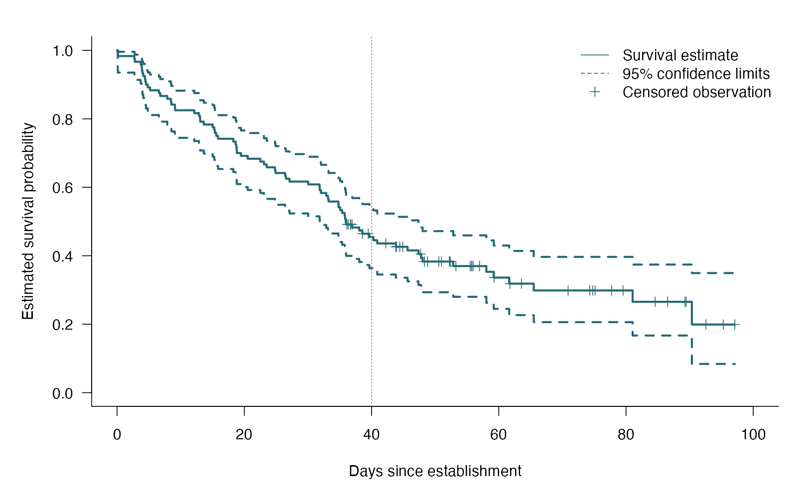
- 120 seedlings; 79 events; 41 censored
- Estimated survival at day 40 = 0.455
- 95% CI 0.364 to 0.542
- Still at risk at day 40: 48
Estimated day-40 survival was 45.5% (95% CI 36.4% to 54.2%), with 48 seedlings still at risk. Kaplan–Meier estimates survival rather than testing a null. Censored seedlings contribute information until their final follow-up; they are not assumed to survive forever.
**Teaching point:** Censored observations contribute until follow-up ends; no invented p-value is needed for estimation.
### Analysis code excerpt
```r
d <- read.csv("modules/kaplan_meier/generated/data.csv")
fit <- survival::survfit(survival::Surv(days, event) ~ 1,
data = d, conf.type = "log-log")
at_day40 <- summary(fit, times = 40)
print(at_day40)
```
The full script supplies package loading and any additional preparation.
### Full printed R output
```text
Call: survfit(formula = survival::Surv(days, event) ~ 1, data = d,
conf.type = "log-log")
time n.risk n.event survival std.err lower 95% CI upper 95% CI
0.106 120 1 0.992 0.0083 0.942 0.999
0.126 119 1 0.983 0.0117 0.935 0.996
2.720 118 1 0.975 0.0143 0.925 0.992
2.786 117 1 0.967 0.0164 0.914 0.987
3.710 116 1 0.958 0.0182 0.903 0.982
3.869 115 1 0.950 0.0199 0.892 0.977
3.900 114 1 0.942 0.0214 0.882 0.972
3.983 113 1 0.933 0.0228 0.871 0.966
4.104 112 1 0.925 0.0240 0.861 0.960
4.377 111 1 0.917 0.0252 0.851 0.954
4.446 110 1 0.908 0.0263 0.841 0.948
4.531 109 1 0.900 0.0274 0.831 0.942
4.822 108 1 0.892 0.0284 0.821 0.936
5.181 107 1 0.883 0.0293 0.811 0.929
6.574 106 1 0.875 0.0302 0.801 0.923
6.788 105 1 0.867 0.0310 0.792 0.916
7.888 104 1 0.858 0.0318 0.782 0.909
8.457 103 1 0.850 0.0326 0.773 0.903
8.532 102 1 0.842 0.0333 0.763 0.896
9.082 101 1 0.833 0.0340 0.754 0.889
9.103 100 1 0.825 0.0347 0.744 0.882
12.133 99 1 0.817 0.0353 0.735 0.875
12.867 98 1 0.808 0.0359 0.726 0.868
13.038 97 1 0.800 0.0365 0.717 0.861
13.059 96 1 0.792 0.0371 0.707 0.854
13.633 95 1 0.783 0.0376 0.698 0.847
15.020 94 1 0.775 0.0381 0.689 0.840
15.281 93 1 0.767 0.0386 0.680 0.833
15.370 92 1 0.758 0.0391 0.671 0.825
15.590 91 1 0.750 0.0395 0.662 0.818
15.865 90 1 0.742 0.0400 0.653 0.811
18.267 89 1 0.733 0.0404 0.645 0.803
18.634 88 1 0.725 0.0408 0.636 0.796
18.744 87 1 0.717 0.0411 0.627 0.788
18.800 86 1 0.708 0.0415 0.618 0.781
18.822 85 1 0.700 0.0418 0.609 0.773
19.473 84 1 0.692 0.0422 0.601 0.766
20.529 83 1 0.683 0.0425 0.592 0.758
22.516 82 1 0.675 0.0428 0.583 0.751
23.080 81 1 0.667 0.0430 0.575 0.743
23.526 80 1 0.658 0.0433 0.566 0.736
24.822 79 1 0.650 0.0435 0.558 0.728
24.903 78 1 0.642 0.0438 0.549 0.720
26.414 77 1 0.633 0.0440 0.540 0.712
26.537 76 1 0.625 0.0442 0.532 0.705
27.108 75 1 0.617 0.0444 0.523 0.697
30.038 74 1 0.608 0.0446 0.515 0.689
31.827 73 1 0.600 0.0447 0.507 0.681
31.855 72 1 0.592 0.0449 0.498 0.673
32.051 71 1 0.583 0.0450 0.490 0.666
32.881 70 1 0.575 0.0451 0.482 0.658
33.146 69 1 0.567 0.0452 0.473 0.650
33.241 68 1 0.558 0.0453 0.465 0.642
34.796 67 1 0.550 0.0454 0.457 0.634
34.815 66 1 0.542 0.0455 0.448 0.626
35.056 65 1 0.533 0.0455 0.440 0.618
35.379 64 1 0.525 0.0456 0.432 0.610
35.787 63 1 0.517 0.0456 0.424 0.602
35.834 62 1 0.508 0.0456 0.416 0.594
35.927 61 1 0.500 0.0456 0.408 0.585
35.995 60 1 0.492 0.0456 0.400 0.577
36.970 54 1 0.483 0.0457 0.391 0.568
38.069 53 1 0.473 0.0457 0.382 0.560
38.550 52 1 0.464 0.0457 0.373 0.551
39.659 49 1 0.455 0.0458 0.364 0.542
40.280 48 1 0.445 0.0458 0.354 0.532
40.896 47 1 0.436 0.0458 0.345 0.523
43.820 45 1 0.426 0.0458 0.336 0.514
45.663 40 1 0.416 0.0459 0.325 0.503
47.372 39 1 0.405 0.0459 0.315 0.493
47.792 37 1 0.394 0.0460 0.304 0.483
48.030 36 1 0.383 0.0460 0.293 0.472
52.841 29 1 0.370 0.0462 0.280 0.460
58.048 22 1 0.353 0.0471 0.262 0.445
59.211 21 1 0.336 0.0478 0.245 0.430
61.635 19 1 0.319 0.0484 0.227 0.414
65.496 16 1 0.299 0.0493 0.206 0.397
81.042 9 1 0.265 0.0538 0.167 0.374
90.357 4 1 0.199 0.0702 0.084 0.349
```
### Recreate the observations
```r
output_dir <- "modules/kaplan_meier/generated"
dir.create(output_dir, recursive = TRUE, showWarnings = FALSE)
set.seed(2110)
d <- data.frame(seedling = 1:120)
event_time <- rexp(120, rate = .018)
follow_up <- runif(120, 35, 100)
d$days <- pmin(event_time, follow_up)
d$event <- as.integer(event_time <= follow_up)
write.csv(d, file.path(output_dir, "data.csv"), row.names = FALSE)
```
Run the complete module from the course folder:
```sh
Rscript modules/kaplan_meier/analysis.R modules/kaplan_meier/generated
```
## Dataset 48: Log-rank survival comparison
Plant pathologists compare time to infection under three protective treatments.
**Family:** Time to event · **Rows:** 150 · **Seed:** 2111
[Saved CSV](modules/log_rank/generated/data.csv) · [Full runnable R script](modules/log_rank/analysis.R) · [Full-size plot](modules/log_rank/generated/plot.png)
**Generating truth:** Equal survival is false: day-30 infection-free probabilities are exp(−1.35) ≈ 0.259, exp(−0.9) ≈ 0.407 and exp(−0.54) ≈ 0.583. The high/control hazard ratio is 0.4, though the log-rank test itself does not estimate it.
**Exact generating model:** 50 independent plants per group have exponential infection times with rates 0.045, 0.030 and 0.018/day in Control, Low and High treatment. Independent follow-up is Uniform(40, 80) days. Save the minimum time and an event indicator; no rounding. The construction gives proportional hazards and noninformative censoring.
**Scientific question:** Are the infection-free survival curves equal across treatments?
**Null being tested / estimation target:** The groups have the same survival function over follow-up.
**Design and independent unit:** 50 independent plants per treatment; some plants remain uninfected at final follow-up.
### Columns
| Column | Meaning | Unit / type |
|---|---|---|
| plant | Independent plant identifier | ID |
| treatment | Protective treatment level | category |
| days | Time to infection or last follow-up | day |
| event | 1 infection; 0 right-censored | binary |
### Analysis from the saved dataset
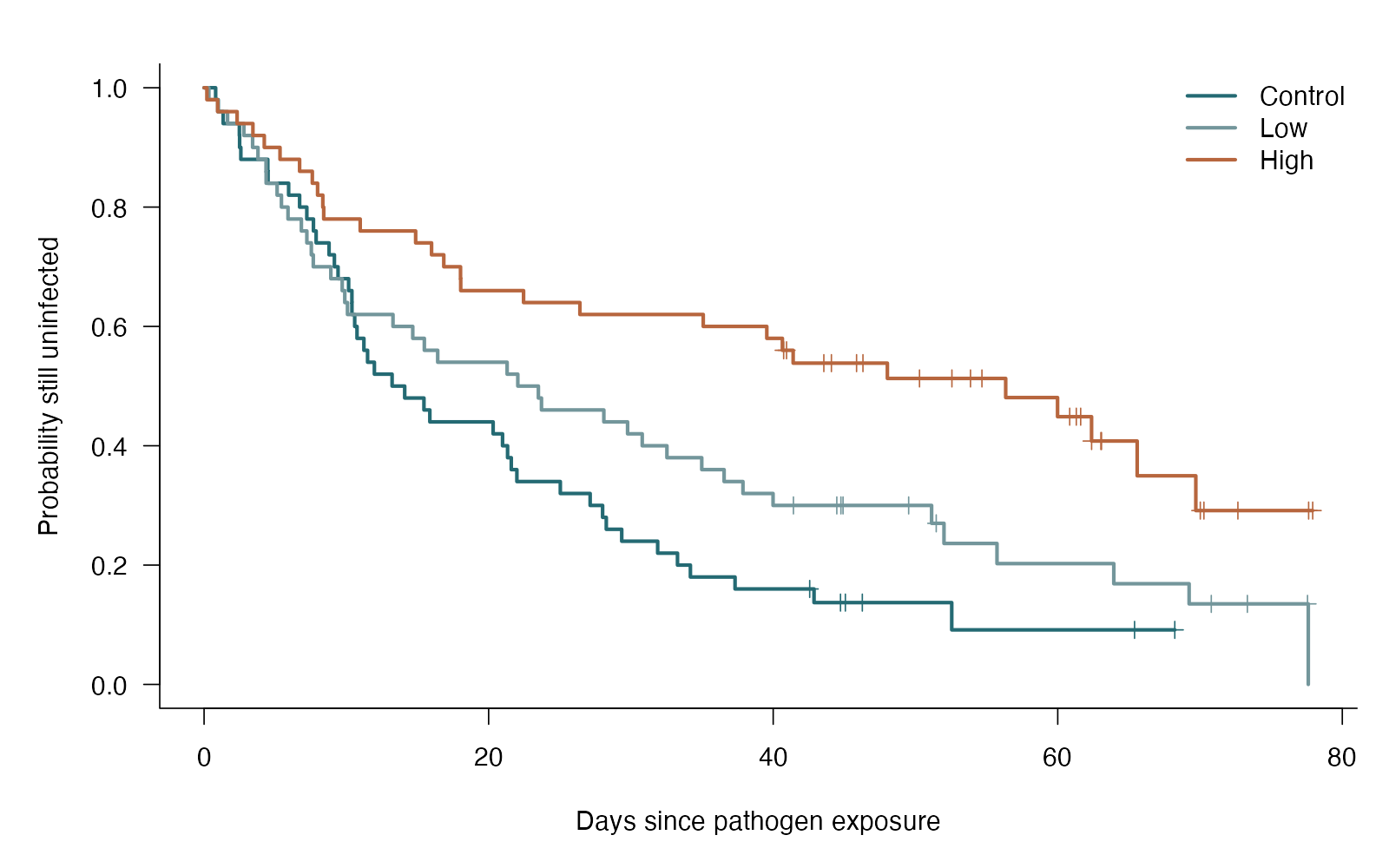
- Log-rank chi-square(2) = 17.18
- Omnibus p = 0.0001863
- Control day-30 survival 0.24 (95% CI 0.15–0.39)
- High day-30 survival 0.62 (95% CI 0.50–0.77)
The three infection-free survival curves differed (log-rank chi-square(2) = 17.18, p = 0.0001863). Estimated day-30 infection-free fractions were 0.24 in control and 0.62 in high treatment. The omnibus test does not identify each differing pair and does not estimate a hazard ratio.
**Teaching point:** An omnibus survival comparison is not a pairwise effect estimate.
### Analysis code excerpt
```r
d <- read.csv("modules/log_rank/generated/data.csv")
test <- survival::survdiff(survival::Surv(days, event) ~ treatment,
data = d, rho = 0)
fit <- survival::survfit(survival::Surv(days, event) ~ treatment, data = d)
p_value <- pchisq(test$chisq, df = length(test$n) - 1, lower.tail = FALSE)
```
The full script supplies package loading and any additional preparation.
### Full printed R output
```text
Call: survfit(formula = survival::Surv(days, event) ~ treatment, data = d)
treatment=Control
time n.risk n.event survival std.err lower 95% CI upper 95% CI
0.813 50 1 0.9800 0.0198 0.9420 1.000
0.992 49 1 0.9600 0.0277 0.9072 1.000
1.344 48 1 0.9400 0.0336 0.8764 1.000
2.481 47 1 0.9200 0.0384 0.8478 0.998
2.498 46 1 0.9000 0.0424 0.8206 0.987
2.584 45 1 0.8800 0.0460 0.7944 0.975
4.478 44 1 0.8600 0.0491 0.7690 0.962
4.495 43 1 0.8400 0.0518 0.7443 0.948
5.943 42 1 0.8200 0.0543 0.7201 0.934
6.715 41 1 0.8000 0.0566 0.6965 0.919
7.222 40 1 0.7800 0.0586 0.6732 0.904
7.687 39 1 0.7600 0.0604 0.6504 0.888
7.875 38 1 0.7400 0.0620 0.6279 0.872
8.784 37 1 0.7200 0.0635 0.6057 0.856
9.159 36 1 0.7000 0.0648 0.5838 0.839
9.416 35 1 0.6800 0.0660 0.5623 0.822
10.160 34 1 0.6600 0.0670 0.5409 0.805
10.390 33 1 0.6400 0.0679 0.5199 0.788
10.392 32 1 0.6200 0.0686 0.4991 0.770
10.587 31 1 0.6000 0.0693 0.4785 0.752
10.749 30 1 0.5800 0.0698 0.4581 0.734
11.233 29 1 0.5600 0.0702 0.4380 0.716
11.492 28 1 0.5400 0.0705 0.4181 0.697
11.969 27 1 0.5200 0.0707 0.3984 0.679
13.215 26 1 0.5000 0.0707 0.3790 0.660
14.101 25 1 0.4800 0.0707 0.3597 0.641
15.453 24 1 0.4600 0.0705 0.3407 0.621
15.867 23 1 0.4400 0.0702 0.3218 0.602
20.316 22 1 0.4200 0.0698 0.3032 0.582
20.978 21 1 0.4000 0.0693 0.2849 0.562
21.332 20 1 0.3800 0.0686 0.2667 0.541
21.591 19 1 0.3600 0.0679 0.2488 0.521
21.986 18 1 0.3400 0.0670 0.2311 0.500
25.038 17 1 0.3200 0.0660 0.2136 0.479
27.135 16 1 0.3000 0.0648 0.1964 0.458
28.011 15 1 0.2800 0.0635 0.1795 0.437
28.269 14 1 0.2600 0.0620 0.1629 0.415
29.354 13 1 0.2400 0.0604 0.1466 0.393
31.881 12 1 0.2200 0.0586 0.1305 0.371
33.274 11 1 0.2000 0.0566 0.1149 0.348
34.181 10 1 0.1800 0.0543 0.0996 0.325
37.319 9 1 0.1600 0.0518 0.0848 0.302
42.870 7 1 0.1371 0.0492 0.0679 0.277
52.549 3 1 0.0914 0.0497 0.0315 0.265
treatment=Low
time n.risk n.event survival std.err lower 95% CI upper 95% CI
0.336 50 1 0.980 0.0198 0.9420 1.000
0.962 49 1 0.960 0.0277 0.9072 1.000
1.650 48 1 0.940 0.0336 0.8764 1.000
2.796 47 1 0.920 0.0384 0.8478 0.998
3.411 46 1 0.900 0.0424 0.8206 0.987
3.787 45 1 0.880 0.0460 0.7944 0.975
4.355 44 1 0.860 0.0491 0.7690 0.962
4.363 43 1 0.840 0.0518 0.7443 0.948
5.133 42 1 0.820 0.0543 0.7201 0.934
5.437 41 1 0.800 0.0566 0.6965 0.919
5.899 40 1 0.780 0.0586 0.6732 0.904
6.838 39 1 0.760 0.0604 0.6504 0.888
7.224 38 1 0.740 0.0620 0.6279 0.872
7.538 37 1 0.720 0.0635 0.6057 0.856
7.675 36 1 0.700 0.0648 0.5838 0.839
8.909 35 1 0.680 0.0660 0.5623 0.822
9.707 34 1 0.660 0.0670 0.5409 0.805
9.890 33 1 0.640 0.0679 0.5199 0.788
10.080 32 1 0.620 0.0686 0.4991 0.770
13.278 31 1 0.600 0.0693 0.4785 0.752
14.667 30 1 0.580 0.0698 0.4581 0.734
15.481 29 1 0.560 0.0702 0.4380 0.716
16.421 28 1 0.540 0.0705 0.4181 0.697
21.299 27 1 0.520 0.0707 0.3984 0.679
22.051 26 1 0.500 0.0707 0.3790 0.660
23.496 25 1 0.480 0.0707 0.3597 0.641
23.714 24 1 0.460 0.0705 0.3407 0.621
28.097 23 1 0.440 0.0702 0.3218 0.602
29.766 22 1 0.420 0.0698 0.3032 0.582
30.795 21 1 0.400 0.0693 0.2849 0.562
32.531 20 1 0.380 0.0686 0.2667 0.541
34.979 19 1 0.360 0.0679 0.2488 0.521
36.550 18 1 0.340 0.0670 0.2311 0.500
37.875 17 1 0.320 0.0660 0.2136 0.479
39.991 16 1 0.300 0.0648 0.1964 0.458
51.134 10 1 0.270 0.0649 0.1686 0.432
52.005 8 1 0.236 0.0650 0.1378 0.405
55.730 7 1 0.202 0.0639 0.1091 0.376
63.940 6 1 0.169 0.0615 0.0826 0.345
69.234 5 1 0.135 0.0577 0.0584 0.312
77.609 1 1 0.000 NaN NA NA
treatment=High
time n.risk n.event survival std.err lower 95% CI upper 95% CI
0.198 50 1 0.980 0.0198 0.942 1.000
0.954 49 1 0.960 0.0277 0.907 1.000
2.322 48 1 0.940 0.0336 0.876 1.000
3.432 47 1 0.920 0.0384 0.848 0.998
4.231 46 1 0.900 0.0424 0.821 0.987
5.337 45 1 0.880 0.0460 0.794 0.975
6.714 44 1 0.860 0.0491 0.769 0.962
7.608 43 1 0.840 0.0518 0.744 0.948
7.978 42 1 0.820 0.0543 0.720 0.934
8.346 41 1 0.800 0.0566 0.696 0.919
8.408 40 1 0.780 0.0586 0.673 0.904
10.973 39 1 0.760 0.0604 0.650 0.888
14.870 38 1 0.740 0.0620 0.628 0.872
15.989 37 1 0.720 0.0635 0.606 0.856
16.848 36 1 0.700 0.0648 0.584 0.839
18.024 35 1 0.680 0.0660 0.562 0.822
18.038 34 1 0.660 0.0670 0.541 0.805
22.455 33 1 0.640 0.0679 0.520 0.788
26.415 32 1 0.620 0.0686 0.499 0.770
35.083 31 1 0.600 0.0693 0.478 0.752
39.551 30 1 0.580 0.0698 0.458 0.734
40.646 29 1 0.560 0.0702 0.438 0.716
41.403 26 1 0.538 0.0707 0.416 0.697
48.025 21 1 0.513 0.0719 0.390 0.675
56.342 16 1 0.481 0.0742 0.355 0.651
59.986 15 1 0.449 0.0758 0.322 0.625
62.376 11 1 0.408 0.0792 0.279 0.597
65.583 7 1 0.350 0.0867 0.215 0.568
69.705 6 1 0.291 0.0897 0.159 0.533
Call:
survival::survdiff(formula = survival::Surv(days, event) ~ treatment,
data = d, rho = 0)
N Observed Expected (O-E)^2/E (O-E)^2/V
treatment=Control 50 44 28.8 8.000 11.16
treatment=Low 50 41 36.7 0.515 0.76
treatment=High 50 29 48.5 7.857 14.15
Chisq= 17.2 on 2 degrees of freedom, p= 2e-04
```
### Recreate the observations
```r
output_dir <- "modules/log_rank/generated"
dir.create(output_dir, recursive = TRUE, showWarnings = FALSE)
set.seed(2111)
d <- data.frame(plant = 1:150,
treatment = rep(c("Control", "Low", "High"), each = 50))
event_time <- rexp(150, rate = rep(c(.045, .03, .018), each = 50))
follow_up <- runif(150, 40, 80)
d$days <- pmin(event_time, follow_up)
d$event <- as.integer(event_time <= follow_up)
write.csv(d, file.path(output_dir, "data.csv"), row.names = FALSE)
```
Run the complete module from the course folder:
```sh
Rscript modules/log_rank/analysis.R modules/log_rank/generated
```
## Dataset 49: Stratified log-rank test
Larval survival under stress is compared within 12 rearing blocks.
**Family:** Survival · **Rows:** 120 · **Seed:** 240501
[Saved CSV](modules/stratified_logrank/generated/data.csv) · [Full runnable R script](modules/stratified_logrank/analysis.R) · [Full-size plot](modules/stratified_logrank/generated/plot.png)
**Generating truth:** Stress has a true hazard ratio of 1.6 within each block; the within-block equality null is false.
**Exact generating model:** 120 independent exponential event times conditional on 12 fixed block rates evenly spaced from 0.025 to 0.08 per day. Stress multiplies every block rate by 1.6. Follow-up stops at 30 days.
**Scientific question:** Do matched groups differ in survival after accounting for the matching strata?
**Null being tested / estimation target:** Within the specified strata, groups have the same survival function.
**Design and independent unit:** Independent larvae within known rearing blocks; administrative censoring at day 30.
### Columns
| Column | Meaning | Unit / type |
|---|---|---|
| stratum | Rearing block | ID |
| treatment | Assigned condition | category |
| time | Observed event or censoring time | days |
| event | Event observed by day 30 | TRUE/FALSE |
### Analysis from the saved dataset
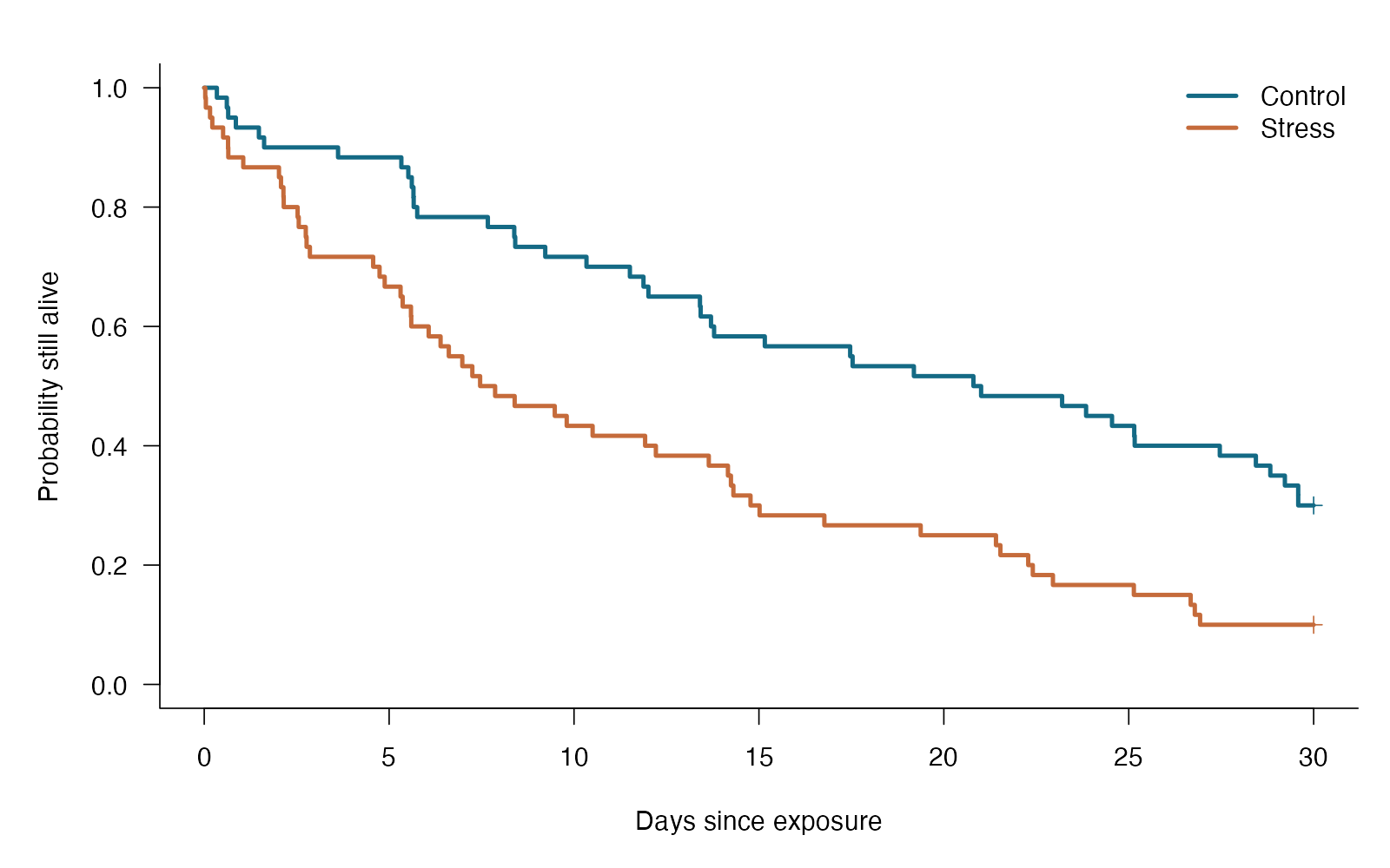
- Stratified chi-square = 13.433
- p = 0.0002472
- 12 rearing blocks; 120 larvae
After comparison within rearing blocks, chi-square = 13.43 (1 df), p = 0.000247. The test compares survival; estimate the direction and magnitude with survival curves or a suitable model.
**Teaching point:** Stratification permits different baseline survival across known blocks.
### Analysis code excerpt
```r
d <- read.csv("modules/stratified_logrank/generated/data.csv")
result <- survival::survdiff(survival::Surv(time, event) ~ treatment + strata(stratum), data=d)
p_value <- pchisq(result$chisq, df=1, lower.tail=FALSE)
```
The full script supplies package loading and any additional preparation.
### Full printed R output
```text
Call:
survival::survdiff(formula = survival::Surv(time, event) ~ treatment +
strata(stratum), data = d)
N Observed Expected (O-E)^2/E (O-E)^2/V
treatment=Control 60 42 58.5 4.64 13.4
treatment=Stress 60 54 37.5 7.23 13.4
Chisq= 13.4 on 1 degrees of freedom, p= 2e-04
```
### Recreate the observations
```r
out_dir <- "modules/stratified_logrank/generated"
dir.create(out_dir, recursive = TRUE, showWarnings = FALSE)
set.seed(240501)
stratum <- rep(1:12, each=10)
treatment <- rep(rep(c("Control", "Stress"), each=5), 12)
rate <- rep(seq(.025, .08, length.out=12), each=10)
event_time <- rexp(120, rate * ifelse(treatment=="Stress", 1.6, 1))
d <- data.frame(stratum, treatment, time=pmin(event_time, 30), event=event_time<=30)
write.csv(d, file.path(out_dir, "data.csv"), row.names = FALSE)
```
Run the complete module from the course folder:
```sh
Rscript modules/stratified_logrank/analysis.R modules/stratified_logrank/generated
```
## Dataset 50: Cox proportional-hazards regression
Seedling death times are related to protective dose and temperature.
**Family:** Time to event · **Rows:** 180 · **Seed:** 2112
[Saved CSV](modules/cox_ph/generated/data.csv) · [Full runnable R script](modules/cox_ph/analysis.R) · [Full-size plot](modules/cox_ph/generated/plot.png)
**Generating truth:** The adjusted hazard ratio per dose unit is exp(−0.45) ≈ 0.638; per °C it is exp(0.12) ≈ 1.127. The dose null is false and proportional hazards holds in the generating model.
**Exact generating model:** 180 seedlings have dose Uniform(0, 3) and temperature Normal(25, 2²)°C. Conditional event times are exponential with rate exp(log(0.035) − 0.45 × dose + 0.12 × (temperature − 25)). Independent censoring times are Uniform(45, 100) days. Save the minimum time and event indicator without rounding.
**Scientific question:** Does dose alter death hazard after accounting for temperature?
**Null being tested / estimation target:** The dose coefficient is zero: the adjusted hazard ratio per dose unit is one.
**Design and independent unit:** 180 independent seedlings with right-censoring.
### Columns
| Column | Meaning | Unit / type |
|---|---|---|
| seedling | Independent seedling identifier | ID |
| dose | Protective dose | dose unit |
| temperature | Rearing temperature | °C |
| days | Observed death or censoring time | day |
| event | 1 death; 0 right-censored | binary |
### Analysis from the saved dataset
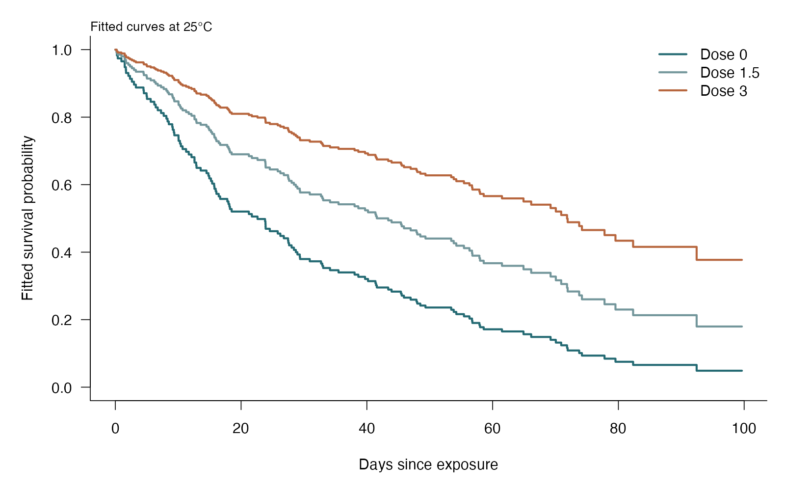
- Dose hazard ratio per unit = 0.69
- 95% CI 0.56 to 0.84
- Wald z = -3.72; p = 0.0001969
- PH diagnostic global p = 0.01934
Each dose unit multiplied the death hazard by 0.69 at the same temperature (95% CI 0.56 to 0.84; Wald p = 0.0001969). This is an instantaneous-risk comparison among seedlings still alive, not a survival probability ratio. The fitted constant hazard ratio must be checked over time.
**Teaching point:** A hazard ratio compares instantaneous event risk among individuals still at risk.
### Analysis code excerpt
```r
d <- read.csv("modules/cox_ph/generated/data.csv")
fit <- survival::coxph(survival::Surv(days, event) ~ dose + temperature,
data = d, x = TRUE)
summary(fit)
ph_check <- survival::cox.zph(fit)
hazard_ci <- exp(confint(fit)["dose", ])
```
The full script supplies package loading and any additional preparation.
### Full printed R output
```text
Call:
survival::coxph(formula = survival::Surv(days, event) ~ dose +
temperature, data = d, x = TRUE)
n= 180, number of events= 126
coef exp(coef) se(coef) z Pr(>|z|)
dose -0.37705 0.68588 0.10128 -3.723 0.000197 ***
temperature 0.16013 1.17367 0.04852 3.300 0.000966 ***
---
Signif. codes: 0 ‘***’ 0.001 ‘**’ 0.01 ‘*’ 0.05 ‘.’ 0.1 ‘ ’ 1
exp(coef) exp(-coef) lower .95 upper .95
dose 0.6859 1.458 0.5624 0.8365
temperature 1.1737 0.852 1.0672 1.2908
Concordance= 0.628 (se = 0.027 )
Likelihood ratio test= 21.6 on 2 df, p=2e-05
Wald test = 21.43 on 2 df, p=2e-05
Score (logrank) test = 21.27 on 2 df, p=2e-05
chisq df p
dose 7.726 1 0.0054
temperature 0.942 1 0.3317
GLOBAL 7.891 2 0.0193
```
### Recreate the observations
```r
output_dir <- "modules/cox_ph/generated"
dir.create(output_dir, recursive = TRUE, showWarnings = FALSE)
set.seed(2112)
d <- data.frame(seedling = 1:180, dose = runif(180, 0, 3),
temperature = rnorm(180, 25, 2))
rate <- exp(log(.035) - .45 * d$dose + .12 * (d$temperature - 25))
event_time <- rexp(180, rate = rate)
follow_up <- runif(180, 45, 100)
d$days <- pmin(event_time, follow_up)
d$event <- as.integer(event_time <= follow_up)
write.csv(d, file.path(output_dir, "data.csv"), row.names = FALSE)
```
Run the complete module from the course folder:
```sh
Rscript modules/cox_ph/analysis.R modules/cox_ph/generated
```
## Dataset 51: Parametric survival: accelerated failure time
Botanists compare germination timing after control or cold treatment.
**Family:** Time to event · **Rows:** 140 · **Seed:** 2113
[Saved CSV](modules/parametric_survival/generated/data.csv) · [Full runnable R script](modules/parametric_survival/analysis.R) · [Full-size plot](modules/parametric_survival/generated/plot.png)
**Generating truth:** The population cold/control time ratio is exp(0.4) ≈ 1.492, so the equal-time null is false. The generating Weibull distribution matches the fitted AFT family.
**Exact generating model:** 140 independent seeds (70 per group) have Weibull germination times with shape 1.8 and scale exp(log(20) + 0.4 if Cold). Thus control scale is 20 days and cold scale is about 29.84 days. Independent censoring times are Uniform(22, 50) days. Save minimum time and event indicator without rounding.
**Scientific question:** Does cold treatment stretch the germination-time distribution?
**Null being tested / estimation target:** The treatment coefficient is zero: the cold/control time ratio is one.
**Design and independent unit:** 140 independent seeds; some remain ungerminated at final follow-up.
### Columns
| Column | Meaning | Unit / type |
|---|---|---|
| seed | Independent seed identifier | ID |
| treatment | Control or cold pretreatment | category |
| days | Observed germination or censoring time | day |
| event | 1 germinated; 0 right-censored | binary |
### Analysis from the saved dataset
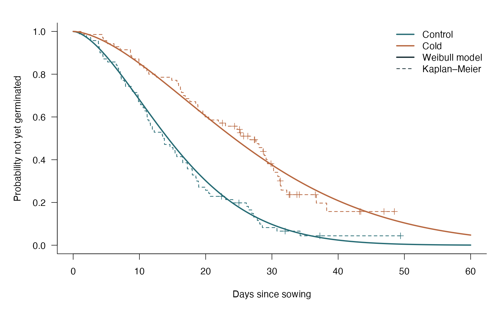
- Cold/control time ratio = 1.70
- 95% CI 1.35 to 2.13
- Wald z = 4.54; p = 5.745e-06
- Fitted Weibull shape = 1.64
Under the Weibull accelerated-failure-time model, cold-treated seeds had 1.70 times the germination time of controls (95% CI 1.35 to 2.13; p = 5.745e-06). This is a time ratio, not a Cox hazard ratio. The distributional fit and censoring assumptions remain part of the interpretation.
**Teaching point:** An AFT coefficient becomes a time ratio; it is not interpreted as a Cox hazard ratio.
### Analysis code excerpt
```r
d <- read.csv("modules/parametric_survival/generated/data.csv")
fit <- survival::survreg(survival::Surv(days, event) ~ treatment,
data = d, dist = "weibull")
summary(fit)
time_ci <- exp(confint(fit)["treatmentCold", ])
```
The full script supplies package loading and any additional preparation.
### Full printed R output
```text
Call:
survival::survreg(formula = survival::Surv(days, event) ~ treatment,
data = d, dist = "weibull")
Value Std. Error z p
(Intercept) 2.8854 0.0773 37.32 < 2e-16
treatmentCold 0.5288 0.1166 4.54 5.7e-06
Log(scale) -0.4935 0.0759 -6.50 8.1e-11
Scale= 0.61
Weibull distribution
Loglik(model)= -454.6 Loglik(intercept only)= -465
Chisq= 20.72 on 1 degrees of freedom, p= 5.3e-06
Number of Newton-Raphson Iterations: 5
n= 140
```
### Recreate the observations
```r
output_dir <- "modules/parametric_survival/generated"
dir.create(output_dir, recursive = TRUE, showWarnings = FALSE)
set.seed(2113)
d <- data.frame(seed = 1:140,
treatment = rep(c("Control", "Cold"), each = 70))
log_scale <- log(20) + .4 * (d$treatment == "Cold")
event_time <- rweibull(140, shape = 1.8, scale = exp(log_scale))
follow_up <- runif(140, 22, 50)
d$days <- pmin(event_time, follow_up)
d$event <- as.integer(event_time <= follow_up)
write.csv(d, file.path(output_dir, "data.csv"), row.names = FALSE)
```
Run the complete module from the course folder:
```sh
Rscript modules/parametric_survival/analysis.R modules/parametric_survival/generated
```
## Dataset 52: Shared-frailty survival model
Larvae from 24 populations experience a control or stress condition.
**Family:** Survival · **Rows:** 240 · **Seed:** 240502
[Saved CSV](modules/shared_frailty/generated/data.csv) · [Full runnable R script](modules/shared_frailty/analysis.R) · [Full-size plot](modules/shared_frailty/generated/plot.png)
**Generating truth:** The conditional stress hazard ratio is exp(0.5) ≈ 1.65; shared population variance is 0.5.
**Exact generating model:** 24 population frailties follow Gamma(shape=2, rate=2), mean 1. Conditional event times are exponential with rate 0.04 × frailty × exp(0.5 × stress). Ten larvae per population; censoring at 35 days.
**Scientific question:** Does stress change larval death hazard after accounting for shared population conditions?
**Null being tested / estimation target:** The stress coefficient is zero: the hazard ratio conditional on population frailty is one.
**Design and independent unit:** Larvae share an unobserved population risk; time-to-death is censored at day 35.
### Columns
| Column | Meaning | Unit / type |
|---|---|---|
| population | Shared risk group | ID |
| stress | Control=0, stress=1 | indicator |
| time | Observed follow-up | days |
| event | Death observed | TRUE/FALSE |
### Analysis from the saved dataset
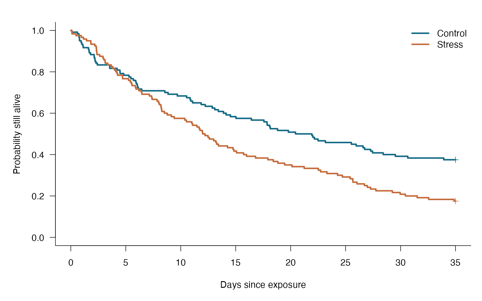
- Conditional hazard ratio = 1.61
- Wald 95% CI 1.18 to 2.18
- Wald p = 0.002373
Stress has an estimated hazard ratio of 1.61 conditional on population frailty (95% Wald CI 1.18 to 2.18; p = 0.00237). Population frailty represents shared differences in baseline risk.
**Teaching point:** Frailty accounts for shared latent risk; it is different from giving each stratum its own baseline curve.
### Analysis code excerpt
```r
d <- read.csv("modules/shared_frailty/generated/data.csv")
result <- survival::coxph(survival::Surv(time, event) ~ stress + frailty(population), data=d)
b <- coef(result)["stress"]
se <- sqrt(vcov(result)["stress", "stress"])
hr <- exp(b); ci <- exp(b+c(-1,1)*1.96*se)
p_value <- 2*pnorm(-abs(b/se))
```
The full script supplies package loading and any additional preparation.
### Full printed R output
```text
Call:
survival::coxph(formula = survival::Surv(time, event) ~ stress +
frailty(population), data = d)
coef se(coef) se2 Chisq DF p
stress 0.475 0.156 0.155 9.236 1.0 0.0024
frailty(population) 55.288 17.2 6.8e-06
Iterations: 8 outer, 31 Newton-Raphson
Variance of random effect= 0.337 I-likelihood = -848
Degrees of freedom for terms= 1.0 17.2
Likelihood ratio test=82.8 on 18.1 df, p=3e-10
n= 240, number of events= 174
```
### Recreate the observations
```r
out_dir <- "modules/shared_frailty/generated"
dir.create(out_dir, recursive = TRUE, showWarnings = FALSE)
set.seed(240502)
population <- rep(1:24, each=10)
stress <- rep(rep(0:1, each=5), 24)
frailty <- rgamma(24, shape=2, rate=2)
event_time <- rexp(240, .04 * frailty[population] * exp(.5*stress))
d <- data.frame(population, stress, time=pmin(event_time, 35), event=event_time<=35)
write.csv(d, file.path(out_dir, "data.csv"), row.names = FALSE)
```
Run the complete module from the course folder:
```sh
Rscript modules/shared_frailty/analysis.R modules/shared_frailty/generated
```
## Dataset 53: Independent-sample permutation test
Independent insect larvae are randomly assigned to ambient or warm rearing.
**Family:** Simulation and multivariate methods · **Rows:** 50 · **Seed:** 240503
[Saved CSV](modules/permutation_independent/generated/data.csv) · [Full runnable R script](modules/permutation_independent/analysis.R) · [Full-size plot](modules/permutation_independent/generated/plot.png)
**Generating truth:** The simulated warm-minus-control mean difference is 1.1 mm; the same-distribution null is false.
**Exact generating model:** 25 independent values per group. Control growth is Normal(8, SD=1.8) mm; warm growth is Normal(9.1, SD=1.8) mm. No rounding or clipping.
**Scientific question:** Would the observed group statistic be unusual under assignments permitted by the design?
**Null being tested / estimation target:** For ordinary group-label permutation, group labels are exchangeable under the null; in a randomized experiment, the sharp null is no treatment effect on any unit.
**Design and independent unit:** Two independent randomized groups; statistic is the mean difference.
### Columns
| Column | Meaning | Unit / type |
|---|---|---|
| group | Randomized treatment | category |
| growth_mm | Larval growth | mm |
### Analysis from the saved dataset
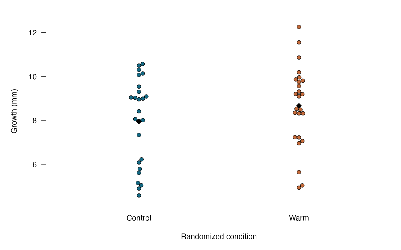
- Warm − control = 0.72 mm
- Two-sided Monte Carlo p = 0.187
- 4999 permitted label shuffles
Mean growth was 0.72 mm higher under warming; the two-sided permutation p-value is 0.187 from 4999 random assignments. The shuffle must match the design.
**Teaching point:** Choose the statistic for the scientific question, then shuffle in a way the design permits.
### Analysis code excerpt
```r
d <- read.csv("modules/permutation_independent/generated/data.csv")
observed <- mean(d$growth_mm[d$group=="Warm"])-mean(d$growth_mm[d$group=="Control"])
B <- 4999
null <- numeric(B)
for (i in 1:B) {
shuffled <- sample(d$group)
null[i] <- mean(d$growth_mm[shuffled=="Warm"])-mean(d$growth_mm[shuffled=="Control"])
}
p_value <- (1+sum(abs(null)>=abs(observed)))/(B+1)
result <- data.frame(mean_difference=observed, permutations=B, p=p_value)
```
The full script supplies package loading and any additional preparation.
### Full printed R output
```text
mean_difference permutations p
1 0.7207885 4999 0.187
```
### Recreate the observations
```r
out_dir <- "modules/permutation_independent/generated"
dir.create(out_dir, recursive = TRUE, showWarnings = FALSE)
set.seed(240503)
group <- rep(c("Control", "Warm"), each=25)
d <- data.frame(group, growth_mm=rnorm(50, 8+1.1*(group=="Warm"), 1.8))
write.csv(d, file.path(out_dir, "data.csv"), row.names = FALSE)
```
Run the complete module from the course folder:
```sh
Rscript modules/permutation_independent/analysis.R modules/permutation_independent/generated
```
## Dataset 54: Paired permutation test
Two comparable leaves per plant receive randomized control or shade treatment.
**Family:** Simulation and multivariate methods · **Rows:** 28 · **Seed:** 240504
[Saved CSV](modules/permutation_paired/generated/data.csv) · [Full runnable R script](modules/permutation_paired/analysis.R) · [Full-size plot](modules/permutation_paired/generated/plot.png)
**Generating truth:** The true mean shaded-minus-control difference is −1.2; plants also differ in their shared baseline.
**Exact generating model:** Plant baselines are Normal(15, SD=2). Independent leaf errors are Normal(0, SD=1). Shading subtracts 1.2 photosynthesis units.
**Scientific question:** Is the within-pair or within-block contrast unusual under the actual randomization?
**Null being tested / estimation target:** Under a paired randomized design, treatment assignment has no effect on any unit; permitted within-pair swaps are equally plausible.
**Design and independent unit:** Matched leaves within 28 independent plants; treatment labels are randomized within each plant.
### Columns
| Column | Meaning | Unit / type |
|---|---|---|
| plant | Independent matched unit | ID |
| control | Control-leaf rate | photosynthesis units |
| shaded | Shaded-leaf rate | photosynthesis units |
### Analysis from the saved dataset
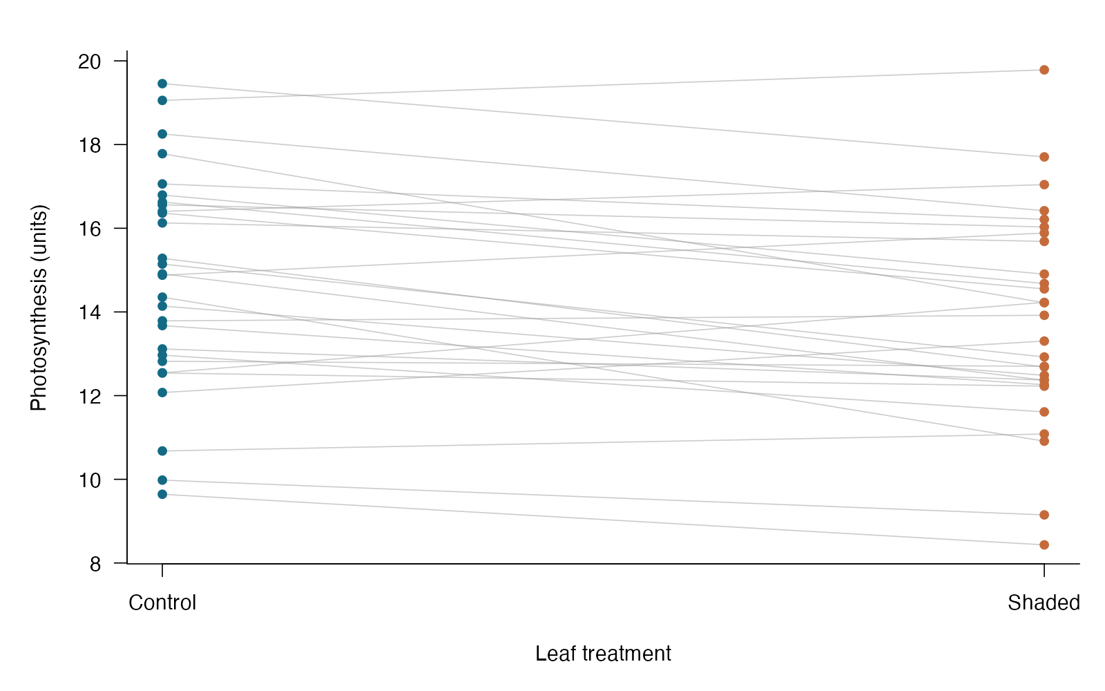
- Shaded − control = -0.97 units
- Two-sided permutation p = 0.0006
- 28 pairs; labels swap only within plants
Within plants, shading changed mean photosynthesis by -0.97 units (paired permutation p = 0.0006). Swaps preserve plant pairing.
**Teaching point:** Swapping labels within a pair is equivalent to reversing the sign of that pair’s difference.
### Analysis code excerpt
```r
d <- read.csv("modules/permutation_paired/generated/data.csv")
difference <- d$shaded-d$control
observed <- mean(difference)
B <- 4999
null <- numeric(B)
for (i in 1:B) null[i] <- mean(difference * sample(c(-1,1), nrow(d), replace=TRUE))
p_value <- (1+sum(abs(null)>=abs(observed)))/(B+1)
result <- data.frame(mean_difference=observed, permutations=B, p=p_value)
```
The full script supplies package loading and any additional preparation.
### Full printed R output
```text
mean_difference permutations p
1 -0.9724543 4999 6e-04
```
### Recreate the observations
```r
out_dir <- "modules/permutation_paired/generated"
dir.create(out_dir, recursive = TRUE, showWarnings = FALSE)
set.seed(240504)
baseline <- rnorm(28, 15, 2)
d <- data.frame(plant=1:28, control=baseline+rnorm(28,0,1),
shaded=baseline-1.2+rnorm(28,0,1))
write.csv(d, file.path(out_dir, "data.csv"), row.names = FALSE)
```
Run the complete module from the course folder:
```sh
Rscript modules/permutation_paired/analysis.R modules/permutation_paired/generated
```
## Dataset 55: Monte Carlo null-model test
Test whether candidate sex-determination genes are unusually concentrated on the X chromosome.
**Family:** Simulation and multivariate methods · **Rows:** 80 · **Seed:** 240505
[Saved CSV](modules/monte_carlo/generated/data.csv) · [Full runnable R script](modules/monte_carlo/analysis.R) · [Full-size plot](modules/monte_carlo/generated/plot.png)
**Generating truth:** The true occupancy probability is 0.32, so the tested 0.20 null is false.
**Exact generating model:** 80 independent Bernoulli indicators with true X probability 0.32. The tested null probability is 0.20; null simulation uses 9999 binomial draws.
**Scientific question:** Is chromosome occupancy inconsistent with the specified opportunity model?
**Null being tested / estimation target:** Each independent candidate gene has probability 0.20 of being on X.
**Design and independent unit:** A teaching null assigns independent genes to X with probability equal to its opportunity share.
### Columns
| Column | Meaning | Unit / type |
|---|---|---|
| gene | Candidate gene | ID |
| on_X | X chromosome=1, other=0 | indicator |
### Analysis from the saved dataset
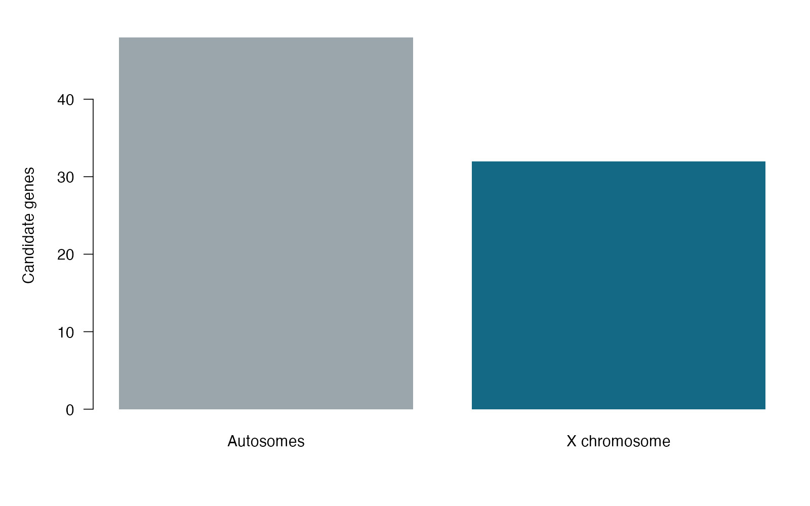
- Observed on X: 32 of 80
- Expected under null: 16.0
- Two-sided Monte Carlo p = 0.0002
32 of 80 genes were on X, compared with null expectation 16.0. The absolute count-deviation Monte Carlo test gives p = 0.0002. Here the null assigns each independent gene probability 0.20 of being on X.
**Teaching point:** A simulation test is only as useful as its biological null model.
### Analysis code excerpt
```r
d <- read.csv("modules/monte_carlo/generated/data.csv")
observed <- sum(d$on_X)
p0 <- .20; n <- nrow(d); B <- 9999
null <- rbinom(B, size=n, prob=p0)
p_value <- (1+sum(abs(null-n*p0)>=abs(observed-n*p0)))/(B+1)
result <- data.frame(observed_X=observed, expected_X=n*p0, monte_carlo_p=p_value)
```
The full script supplies package loading and any additional preparation.
### Full printed R output
```text
observed_X expected_X monte_carlo_p
1 32 16 2e-04
```
### Recreate the observations
```r
out_dir <- "modules/monte_carlo/generated"
dir.create(out_dir, recursive = TRUE, showWarnings = FALSE)
set.seed(240505)
d <- data.frame(gene=1:80, on_X=rbinom(80, 1, .32))
write.csv(d, file.path(out_dir, "data.csv"), row.names = FALSE)
```
Run the complete module from the course folder:
```sh
Rscript modules/monte_carlo/analysis.R modules/monte_carlo/generated
```
## Dataset 56: Bootstrap confidence interval
Estimate average biomass from independent bacterial colonies with a right-skewed distribution.
**Family:** Simulation and multivariate methods · **Rows:** 40 · **Seed:** 240507
[Saved CSV](modules/bootstrap/generated/data.csv) · [Full runnable R script](modules/bootstrap/analysis.R) · [Full-size plot](modules/bootstrap/generated/plot.png)
**Generating truth:** The population arithmetic mean is approximately 13.28 mg; the interval may or may not cover it in one sample.
**Exact generating model:** 40 independent Lognormal(meanlog=log(12), sdlog=0.45) colony biomasses. The generating arithmetic mean is exp(log(12)+0.45^2/2), approximately 13.28 mg.
**Scientific question:** How uncertain is the estimated mean biomass?
**Null being tested / estimation target:** No null is required for this confidence interval; the target is the population mean.
**Design and independent unit:** One biomass measurement per independent colony.
### Columns
| Column | Meaning | Unit / type |
|---|---|---|
| colony | Independent colony | ID |
| biomass_mg | Measured biomass | mg |
### Analysis from the saved dataset
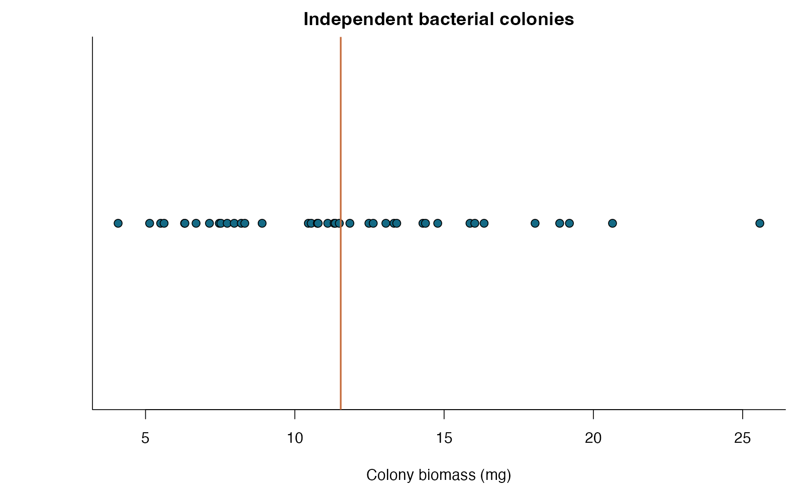
- Sample mean = 11.54 mg
- Percentile 95% CI = 10.15 to 13.07 mg
- 4999 resamples of independent colonies
Mean colony biomass is 11.54 mg, with a percentile bootstrap 95% interval of 10.15 to 13.07 mg. The interval estimates uncertainty in the mean, not the spread of individual colonies.
**Teaching point:** Resampling changes the computational procedure, not what counts as an independent replicate.
### Analysis code excerpt
```r
d <- read.csv("modules/bootstrap/generated/data.csv")
B <- 4999
boot_mean <- numeric(B)
for (i in 1:B) boot_mean[i] <- mean(sample(d$biomass_mg, replace=TRUE))
ci <- quantile(boot_mean, c(.025,.975))
result <- data.frame(mean=mean(d$biomass_mg), lower=ci[1], upper=ci[2])
```
The full script supplies package loading and any additional preparation.
### Full printed R output
```text
mean lower upper
2.5% 11.53829 10.14616 13.06527
```
### Recreate the observations
```r
out_dir <- "modules/bootstrap/generated"
dir.create(out_dir, recursive = TRUE, showWarnings = FALSE)
set.seed(240507)
d <- data.frame(colony=1:40, biomass_mg=rlnorm(40, log(12), .45))
write.csv(d, file.path(out_dir, "data.csv"), row.names = FALSE)
```
Run the complete module from the course folder:
```sh
Rscript modules/bootstrap/analysis.R modules/bootstrap/generated
```
## Dataset 57: Sampling variation and CI coverage
Independent cell cultures differ in the waiting time to a developmental transition.
**Family:** Simulation and multivariate methods · **Rows:** 25000 · **Seed:** 240506
[Saved CSV](modules/sampling_coverage/generated/data.csv) · [Full runnable R script](modules/sampling_coverage/analysis.R) · [Full-size plot](modules/sampling_coverage/generated/plot.png)
**Generating truth:** The population mean is exactly 5 days; nominal 95% coverage is a procedure property to evaluate, not an imposed simulation result.
**Exact generating model:** 1000 samples of 25 independent Exponential(rate=0.2/day) observations. Every sample uses a conventional two-sided 95% t interval for its mean.
**Scientific question:** How often does a stated interval procedure cover the true population mean?
**Null being tested / estimation target:** This is a performance simulation, not a single hypothesis test. The known population mean is 5 days.
**Design and independent unit:** Repeat a 25-cell sampling experiment 1000 times from a known population.
### Columns
| Column | Meaning | Unit / type |
|---|---|---|
| experiment | Repeated simulated sample | ID |
| waiting_days | Time to transition | days |
### Analysis from the saved dataset
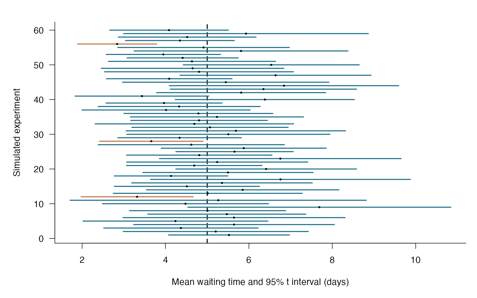
- Mean estimated waiting time: 5.03 days
- Observed 95% t-interval coverage: 92.6%
- True population mean: 5 days
Across 1000 experiments of 25 cells, 92.6% of nominal 95% t intervals contain the true mean of 5 days. Coverage is evaluated against that truth, not each interval’s own sample mean.
**Teaching point:** Larger B stabilizes the estimated coverage; larger n changes the experiment.
### Analysis code excerpt
```r
d <- read.csv("modules/sampling_coverage/generated/data.csv")
low <- high <- estimate <- numeric(1000)
for (i in 1:1000) {
x <- d$waiting_days[d$experiment==i]
estimate[i] <- mean(x)
margin <- qt(.975, length(x)-1)*sd(x)/sqrt(length(x))
low[i] <- mean(x)-margin; high[i] <- mean(x)+margin
}
covered <- low<=5 & high>=5
result <- data.frame(experiment=1:1000, estimate, low, high, covered)
```
The full script supplies package loading and any additional preparation.
### Full printed R output
```text
experiment estimate low high covered
1 1 5.522029 4.072284 6.971773 TRUE
2 2 5.204283 2.985148 7.423418 TRUE
3 3 4.368782 2.517560 6.220003 TRUE
4 4 5.642785 3.234415 8.051154 TRUE
5 5 4.238518 2.021749 6.455288 TRUE
6 6 5.643793 2.979302 8.308284 TRUE
7 7 5.469335 3.573552 7.365119 TRUE
8 8 5.008316 3.136312 6.880320 TRUE
9 9 7.688537 4.535211 10.841862 TRUE
10 10 4.479982 2.489549 6.470416 TRUE
11 11 5.263651 1.711425 8.815877 TRUE
12 12 3.318445 1.975755 4.661135 FALSE
13 13 5.013864 2.746185 7.281543 TRUE
14 14 5.850578 3.541759 8.159396 TRUE
15 15 4.512140 2.771186 6.253094 TRUE
16 16 5.354784 3.188556 7.521012 TRUE
17 17 6.757512 3.640167 9.874857 TRUE
18 18 4.132858 2.769656 5.496059 TRUE
19 19 5.497705 3.455908 7.539502 TRUE
20 20 6.413697 4.247548 8.579845 TRUE
21 21 4.688334 3.063164 6.313503 TRUE
22 22 5.239921 3.067297 7.412546 TRUE
23 23 6.752626 3.853531 9.651721 TRUE
24 24 4.809608 3.067157 6.552059 TRUE
25 25 5.655483 4.247544 7.063422 TRUE
26 26 5.876048 3.895268 7.856828 TRUE
27 27 4.618555 2.384767 6.852343 TRUE
28 28 3.658729 2.417663 4.899794 FALSE
29 29 4.338001 2.857263 5.818739 TRUE
30 30 5.506953 3.072848 7.941058 TRUE
31 31 5.687501 3.054839 8.320163 TRUE
32 32 5.066542 3.191820 6.941265 TRUE
33 33 4.692163 2.311953 7.072373 TRUE
34 34 4.805327 3.165974 6.444680 TRUE
35 35 5.233745 3.158254 7.309237 TRUE
36 36 4.789032 3.003878 6.574186 TRUE
37 37 4.012812 1.996415 6.029208 TRUE
38 38 4.326758 2.382734 6.270782 TRUE
39 39 3.964481 2.574601 5.354360 TRUE
40 40 6.382165 4.232534 8.531796 TRUE
41 41 3.434084 1.829988 5.038180 TRUE
42 42 5.814381 3.787407 7.841355 TRUE
43 43 6.348211 4.113734 8.582688 TRUE
44 44 6.842268 4.091238 9.593298 TRUE
45 45 5.445202 2.970798 7.919606 TRUE
46 46 4.089058 2.582495 5.595621 TRUE
47 47 6.638345 4.348471 8.928219 TRUE
48 48 4.803594 2.537863 7.069326 TRUE
49 49 4.649075 2.458765 6.839386 TRUE
50 50 6.536089 4.425454 8.646724 TRUE
51 51 4.634365 2.627069 6.641661 TRUE
52 52 4.411398 3.077791 5.745006 TRUE
53 53 3.947442 2.577601 5.317284 TRUE
54 54 5.809957 3.245246 8.374669 TRUE
55 55 4.911161 2.853966 6.968356 TRUE
56 56 2.839206 1.888804 3.789608 FALSE
57 57 4.344700 3.039214 5.650185 TRUE
58 58 4.519626 2.867844 6.171408 TRUE
59 59 5.930605 2.995504 8.865706 TRUE
60 60 4.083792 2.659315 5.508269 TRUE
61 61 4.400565 2.899233 5.901897 TRUE
62 62 4.608569 3.206468 6.010671 TRUE
63 63 6.122087 3.529017 8.715158 TRUE
64 64 4.017382 2.632192 5.402571 TRUE
65 65 3.818379 2.364116 5.272641 TRUE
66 66 3.765858 2.317919 5.213796 TRUE
67 67 4.754093 2.844543 6.663642 TRUE
68 68 6.341148 3.941493 8.740803 TRUE
69 69 4.799054 2.697553 6.900555 TRUE
70 70 3.796780 2.443970 5.149590 TRUE
71 71 4.136329 2.731771 5.540887 TRUE
72 72 4.030844 2.327800 5.733889 TRUE
73 73 6.796037 4.119067 9.473006 TRUE
74 74 5.556472 2.973111 8.139833 TRUE
75 75 6.207926 3.910795 8.505058 TRUE
76 76 4.107061 2.152500 6.061622 TRUE
77 77 4.753323 3.124626 6.382020 TRUE
78 78 2.794476 1.369826 4.219126 FALSE
79 79 4.566371 2.837708 6.295035 TRUE
80 80 5.894649 3.659524 8.129775 TRUE
81 81 4.690335 2.896712 6.483958 TRUE
82 82 4.491655 2.640704 6.342605 TRUE
83 83 5.663687 3.229420 8.097953 TRUE
84 84 4.115975 2.707549 5.524400 TRUE
85 85 5.732207 3.571358 7.893057 TRUE
86 86 4.876916 2.965229 6.788603 TRUE
87 87 5.618509 4.067509 7.169509 TRUE
88 88 4.811652 3.344971 6.278334 TRUE
89 89 3.998192 2.273287 5.723097 TRUE
90 90 4.719024 2.958358 6.479690 TRUE
91 91 3.695699 2.389634 5.001764 TRUE
92 92 5.504377 3.267597 7.741157 TRUE
93 93 4.458405 2.330069 6.586741 TRUE
94 94 3.596332 2.582829 4.609835 FALSE
95 95 3.905252 2.464322 5.346181 TRUE
96 96 4.234980 2.561521 5.908438 TRUE
97 97 5.397633 3.101522 7.693744 TRUE
98 98 3.804190 2.235648 5.372732 TRUE
99 99 4.555470 2.447108 6.663832 TRUE
100 100 3.965643 1.957545 5.973742 TRUE
101 101 3.936298 2.425014 5.447583 TRUE
102 102 4.434617 2.475259 6.393976 TRUE
103 103 5.100318 3.290936 6.909700 TRUE
104 104 4.067811 2.542494 5.593129 TRUE
105 105 3.317712 1.908598 4.726826 FALSE
106 106 6.516611 4.021650 9.011571 TRUE
107 107 4.493778 3.003852 5.983703 TRUE
108 108 3.950111 2.552436 5.347785 TRUE
109 109 5.101214 3.126121 7.076308 TRUE
110 110 5.391561 3.582766 7.200356 TRUE
111 111 5.672264 2.436146 8.908382 TRUE
112 112 5.308363 3.405103 7.211624 TRUE
113 113 4.648292 3.070992 6.225592 TRUE
114 114 4.833650 2.986126 6.681173 TRUE
115 115 6.413949 3.788569 9.039328 TRUE
116 116 3.755544 2.547431 4.963657 FALSE
117 117 5.953093 4.095236 7.810951 TRUE
118 118 5.423245 2.814981 8.031510 TRUE
119 119 8.026679 5.101515 10.951842 FALSE
120 120 4.622307 2.434032 6.810582 TRUE
121 121 4.080753 2.700272 5.461233 TRUE
122 122 4.235137 2.645343 5.824930 TRUE
123 123 5.288931 2.278319 8.299543 TRUE
124 124 5.873955 3.016026 8.731884 TRUE
125 125 5.171276 3.380162 6.962391 TRUE
126 126 3.250377 1.489852 5.010902 TRUE
127 127 4.191097 2.668626 5.713568 TRUE
128 128 6.754089 3.601342 9.906836 TRUE
129 129 4.793879 3.097612 6.490145 TRUE
130 130 6.746923 3.533661 9.960186 TRUE
131 131 6.187196 3.894694 8.479698 TRUE
132 132 4.224100 2.524231 5.923970 TRUE
133 133 3.434999 2.221782 4.648216 FALSE
134 134 6.834802 4.139378 9.530226 TRUE
135 135 4.191357 2.319007 6.063707 TRUE
136 136 3.151103 2.060237 4.241968 FALSE
137 137 5.026459 3.169689 6.883229 TRUE
138 138 3.577657 2.528884 4.626430 FALSE
139 139 3.687805 1.994784 5.380827 TRUE
140 140 5.351641 3.422936 7.280347 TRUE
141 141 3.879084 2.304154 5.454013 TRUE
142 142 5.286025 3.516029 7.056022 TRUE
143 143 4.693587 3.300891 6.086283 TRUE
144 144 5.109116 2.401925 7.816308 TRUE
145 145 5.089690 3.333748 6.845632 TRUE
146 146 5.430569 3.870811 6.990327 TRUE
147 147 6.782960 4.339468 9.226452 TRUE
148 148 5.823611 3.331024 8.316199 TRUE
149 149 4.366575 2.390465 6.342684 TRUE
150 150 4.184145 2.110662 6.257627 TRUE
151 151 7.730201 4.354545 11.105856 TRUE
152 152 6.140021 3.348536 8.931505 TRUE
153 153 4.117216 2.409964 5.824468 TRUE
154 154 4.398973 1.430581 7.367365 TRUE
155 155 4.508656 2.892396 6.124916 TRUE
156 156 4.142960 2.664366 5.621555 TRUE
157 157 5.245062 3.098888 7.391237 TRUE
158 158 5.040628 3.008546 7.072711 TRUE
159 159 4.218798 2.480088 5.957507 TRUE
160 160 5.347144 3.433166 7.261123 TRUE
161 161 6.686552 3.977025 9.396078 TRUE
162 162 4.142875 3.147446 5.138305 TRUE
163 163 3.269228 1.170891 5.367566 TRUE
164 164 4.955636 2.996825 6.914446 TRUE
165 165 4.556690 2.991951 6.121429 TRUE
166 166 5.400123 2.910192 7.890054 TRUE
167 167 4.277913 2.393319 6.162508 TRUE
168 168 3.254105 2.029229 4.478981 FALSE
169 169 4.566055 3.025270 6.106840 TRUE
170 170 5.348849 3.080346 7.617352 TRUE
171 171 2.395981 1.556685 3.235278 FALSE
172 172 4.640689 2.748807 6.532571 TRUE
173 173 3.508499 2.009903 5.007095 TRUE
174 174 5.225143 2.841299 7.608988 TRUE
175 175 4.983477 2.784035 7.182919 TRUE
176 176 3.795989 1.917545 5.674432 TRUE
177 177 5.690686 3.581406 7.799967 TRUE
178 178 4.848927 2.914100 6.783754 TRUE
179 179 5.374085 2.260090 8.488080 TRUE
180 180 6.475772 3.811408 9.140136 TRUE
181 181 4.741831 2.402756 7.080906 TRUE
182 182 5.321358 3.240530 7.402186 TRUE
183 183 5.191675 1.921541 8.461809 TRUE
184 184 4.658280 2.766932 6.549628 TRUE
185 185 5.753889 4.188246 7.319532 TRUE
186 186 6.257938 3.073481 9.442395 TRUE
187 187 5.566719 3.929474 7.203964 TRUE
188 188 2.465539 1.547398 3.383681 FALSE
189 189 4.206448 2.561935 5.850961 TRUE
190 190 3.479337 1.933332 5.025342 TRUE
191 191 3.463501 2.085828 4.841174 FALSE
192 192 3.727588 2.093795 5.361380 TRUE
193 193 6.847350 3.846342 9.848358 TRUE
194 194 5.713059 3.598224 7.827895 TRUE
195 195 3.507900 2.070407 4.945393 FALSE
196 196 6.905772 3.535558 10.275986 TRUE
197 197 7.418474 4.791591 10.045357 TRUE
198 198 5.314492 3.311919 7.317065 TRUE
199 199 5.561324 3.223291 7.899358 TRUE
200 200 5.457266 3.586288 7.328244 TRUE
201 201 5.989511 3.791370 8.187652 TRUE
202 202 3.913985 2.508346 5.319624 TRUE
203 203 5.290439 3.427504 7.153373 TRUE
204 204 4.686989 2.752241 6.621737 TRUE
205 205 4.463568 2.682710 6.244426 TRUE
206 206 5.165704 3.407387 6.924021 TRUE
207 207 5.076360 2.702550 7.450170 TRUE
208 208 6.213807 2.760825 9.666789 TRUE
209 209 4.867417 3.309513 6.425321 TRUE
210 210 3.577422 1.434624 5.720220 TRUE
211 211 5.894050 3.514567 8.273532 TRUE
212 212 4.338063 2.560657 6.115469 TRUE
213 213 6.143999 3.323829 8.964169 TRUE
214 214 5.598588 3.768305 7.428870 TRUE
215 215 6.272771 3.983205 8.562336 TRUE
216 216 7.138216 4.579673 9.696759 TRUE
217 217 6.026648 4.078599 7.974697 TRUE
218 218 3.850279 2.341270 5.359289 TRUE
219 219 4.487893 2.978306 5.997479 TRUE
220 220 5.245262 3.003950 7.486574 TRUE
221 221 4.822648 2.948739 6.696558 TRUE
222 222 8.021933 4.637147 11.406719 TRUE
223 223 5.935316 3.847466 8.023167 TRUE
224 224 4.980738 2.542093 7.419382 TRUE
225 225 4.281605 2.961476 5.601734 TRUE
226 226 5.418768 2.691508 8.146029 TRUE
227 227 4.427298 2.528119 6.326477 TRUE
228 228 6.569612 4.002026 9.137198 TRUE
229 229 5.126956 3.152984 7.100928 TRUE
230 230 3.853325 2.401367 5.305283 TRUE
231 231 4.502664 2.540948 6.464380 TRUE
232 232 3.975073 2.580084 5.370062 TRUE
233 233 3.434649 2.342173 4.527125 FALSE
234 234 5.400147 2.760415 8.039879 TRUE
235 235 4.140376 2.134298 6.146454 TRUE
236 236 5.589214 4.041403 7.137025 TRUE
237 237 3.532313 2.393871 4.670754 FALSE
238 238 4.704814 2.780582 6.629047 TRUE
239 239 6.548639 3.403325 9.693952 TRUE
240 240 6.697136 4.277313 9.116959 TRUE
241 241 6.611054 3.033616 10.188492 TRUE
242 242 3.994481 2.210885 5.778078 TRUE
243 243 4.509383 3.090736 5.928030 TRUE
244 244 5.026530 3.017718 7.035342 TRUE
245 245 4.815224 3.105586 6.524861 TRUE
246 246 5.571338 2.475466 8.667209 TRUE
247 247 3.350048 2.078539 4.621557 FALSE
248 248 4.217988 2.648283 5.787692 TRUE
249 249 4.310275 2.014899 6.605652 TRUE
250 250 4.440112 2.616232 6.263992 TRUE
251 251 3.553821 2.381495 4.726146 FALSE
252 252 5.472761 3.405546 7.539975 TRUE
253 253 4.248571 2.281546 6.215597 TRUE
254 254 5.081565 3.002994 7.160135 TRUE
255 255 7.247705 3.855316 10.640094 TRUE
256 256 6.569047 4.377447 8.760647 TRUE
257 257 7.361497 5.158275 9.564720 FALSE
258 258 4.632382 2.402952 6.861812 TRUE
259 259 4.290517 2.594137 5.986896 TRUE
260 260 6.130597 3.595685 8.665509 TRUE
261 261 6.192151 4.400440 7.983862 TRUE
262 262 3.833823 2.241736 5.425911 TRUE
263 263 5.779415 3.498400 8.060429 TRUE
264 264 4.294562 2.340403 6.248721 TRUE
265 265 5.183574 1.892786 8.474362 TRUE
266 266 4.889187 2.752254 7.026119 TRUE
267 267 5.756816 2.918858 8.594774 TRUE
268 268 6.884198 4.169422 9.598975 TRUE
269 269 4.989537 2.320946 7.658129 TRUE
270 270 5.013138 2.522201 7.504074 TRUE
271 271 6.021809 3.395412 8.648207 TRUE
272 272 5.107057 2.865401 7.348712 TRUE
273 273 4.792391 3.209370 6.375412 TRUE
274 274 4.249709 2.221006 6.278412 TRUE
275 275 5.170267 3.380168 6.960365 TRUE
276 276 5.768764 3.080663 8.456865 TRUE
277 277 6.234953 3.083420 9.386486 TRUE
278 278 5.028424 2.781633 7.275215 TRUE
279 279 5.616455 3.487074 7.745837 TRUE
280 280 6.236102 3.960979 8.511224 TRUE
281 281 4.983969 2.177201 7.790738 TRUE
282 282 4.940238 2.891489 6.988987 TRUE
283 283 5.390487 3.274993 7.505981 TRUE
284 284 3.381895 2.098824 4.664966 FALSE
285 285 5.791524 2.618764 8.964283 TRUE
286 286 4.716518 3.311282 6.121754 TRUE
287 287 4.849553 2.268082 7.431024 TRUE
288 288 6.041211 3.583686 8.498735 TRUE
289 289 5.229720 3.264473 7.194968 TRUE
290 290 7.439641 4.404122 10.475160 TRUE
291 291 6.378421 3.828685 8.928157 TRUE
292 292 4.015060 2.681271 5.348850 TRUE
293 293 4.837685 2.984054 6.691316 TRUE
294 294 4.038949 2.735889 5.342009 TRUE
295 295 5.393227 2.732074 8.054380 TRUE
296 296 3.603210 1.905268 5.301151 TRUE
297 297 4.987438 2.865588 7.109287 TRUE
298 298 3.485912 2.313194 4.658630 FALSE
299 299 5.140612 2.954029 7.327194 TRUE
300 300 3.477965 2.236296 4.719633 FALSE
301 301 4.838179 2.666346 7.010013 TRUE
302 302 4.378519 2.904589 5.852448 TRUE
303 303 6.498538 4.652734 8.344341 TRUE
304 304 7.888626 4.962471 10.814781 TRUE
305 305 5.866072 2.703398 9.028746 TRUE
306 306 4.548210 2.879283 6.217138 TRUE
307 307 5.812011 3.232438 8.391584 TRUE
308 308 4.729734 1.924979 7.534489 TRUE
309 309 4.724547 3.012132 6.436962 TRUE
310 310 5.509638 3.535638 7.483638 TRUE
311 311 4.860572 3.116204 6.604940 TRUE
312 312 6.229047 3.491158 8.966936 TRUE
313 313 7.803910 4.373291 11.234530 TRUE
314 314 4.172664 2.392126 5.953202 TRUE
315 315 5.385459 2.042203 8.728715 TRUE
316 316 7.443384 5.117284 9.769484 FALSE
317 317 3.497343 2.049574 4.945112 FALSE
318 318 4.548129 2.747034 6.349224 TRUE
319 319 3.575881 2.061335 5.090426 TRUE
320 320 4.249734 2.824205 5.675263 TRUE
321 321 5.766841 2.901673 8.632008 TRUE
322 322 4.483690 2.292183 6.675196 TRUE
323 323 3.693372 2.348145 5.038599 TRUE
324 324 5.790088 3.547823 8.032353 TRUE
325 325 4.373371 2.672825 6.073916 TRUE
326 326 5.636814 3.126611 8.147018 TRUE
327 327 5.688598 3.445629 7.931566 TRUE
328 328 5.319054 3.285915 7.352192 TRUE
329 329 5.880438 3.824059 7.936816 TRUE
330 330 6.465134 4.247065 8.683202 TRUE
331 331 4.969131 3.396605 6.541658 TRUE
332 332 4.901981 2.672084 7.131878 TRUE
333 333 6.226111 3.711165 8.741058 TRUE
334 334 5.408684 3.786308 7.031060 TRUE
335 335 5.770414 3.100292 8.440535 TRUE
336 336 5.913838 3.614729 8.212947 TRUE
337 337 6.188054 3.866605 8.509502 TRUE
338 338 6.786741 3.736639 9.836843 TRUE
339 339 4.129207 2.361370 5.897044 TRUE
340 340 3.032454 1.717065 4.347843 FALSE
341 341 6.702018 4.001909 9.402128 TRUE
342 342 3.289385 2.287299 4.291471 FALSE
343 343 5.397701 3.036290 7.759112 TRUE
344 344 4.690581 3.338412 6.042750 TRUE
345 345 4.252300 2.408449 6.096151 TRUE
346 346 5.537847 3.517280 7.558414 TRUE
347 347 3.990287 2.845479 5.135095 TRUE
348 348 4.802474 3.107818 6.497130 TRUE
349 349 6.350321 3.977693 8.722949 TRUE
350 350 6.287531 4.145984 8.429079 TRUE
351 351 4.684363 3.022354 6.346373 TRUE
352 352 5.005328 2.055718 7.954937 TRUE
353 353 3.922937 2.744968 5.100905 TRUE
354 354 4.216767 2.555903 5.877632 TRUE
355 355 4.126480 2.520638 5.732323 TRUE
356 356 5.396866 2.614256 8.179475 TRUE
357 357 4.115359 2.418793 5.811926 TRUE
358 358 5.467963 2.648544 8.287381 TRUE
359 359 5.545995 3.918816 7.173173 TRUE
360 360 6.629963 4.361714 8.898212 TRUE
361 361 7.464774 5.190105 9.739443 FALSE
362 362 3.893538 2.313191 5.473885 TRUE
363 363 5.586150 3.581217 7.591083 TRUE
364 364 4.350802 2.798264 5.903340 TRUE
365 365 5.533744 3.580420 7.487067 TRUE
366 366 6.533713 4.433862 8.633563 TRUE
367 367 4.034656 2.408537 5.660776 TRUE
368 368 5.677861 3.199031 8.156691 TRUE
369 369 3.745753 2.345502 5.146004 TRUE
370 370 3.867365 2.604430 5.130300 TRUE
371 371 5.009786 2.314848 7.704724 TRUE
372 372 4.201901 2.228387 6.175415 TRUE
373 373 3.932006 2.575756 5.288256 TRUE
374 374 3.104887 1.706235 4.503538 FALSE
375 375 4.994901 2.689743 7.300058 TRUE
376 376 5.675704 3.555901 7.795507 TRUE
377 377 4.893366 2.777931 7.008801 TRUE
378 378 5.703625 2.303286 9.103965 TRUE
379 379 5.642371 3.428647 7.856096 TRUE
380 380 7.575066 5.039821 10.110312 FALSE
381 381 3.417589 2.028577 4.806602 FALSE
382 382 5.147397 3.561781 6.733013 TRUE
383 383 4.267169 2.690513 5.843826 TRUE
384 384 5.132687 2.856936 7.408438 TRUE
385 385 5.545660 3.562714 7.528607 TRUE
386 386 3.425808 2.099023 4.752593 FALSE
387 387 5.174324 3.301461 7.047187 TRUE
388 388 5.020330 3.321982 6.718679 TRUE
389 389 4.562946 2.850898 6.274993 TRUE
390 390 3.781244 2.000282 5.562206 TRUE
391 391 3.662179 2.277420 5.046939 TRUE
392 392 5.832291 4.107676 7.556906 TRUE
393 393 5.176855 3.283717 7.069992 TRUE
394 394 7.517398 4.950500 10.084297 TRUE
395 395 5.804012 2.897819 8.710204 TRUE
396 396 3.914535 2.172928 5.656142 TRUE
397 397 5.414024 3.584665 7.243382 TRUE
398 398 3.202148 2.113354 4.290942 FALSE
399 399 4.430965 2.894375 5.967554 TRUE
400 400 3.133685 1.751089 4.516282 FALSE
401 401 3.731211 2.333027 5.129395 TRUE
402 402 5.155056 3.787554 6.522558 TRUE
403 403 3.895069 2.278757 5.511381 TRUE
404 404 4.308242 2.671849 5.944635 TRUE
405 405 5.545011 3.640552 7.449471 TRUE
406 406 3.800447 2.172081 5.428814 TRUE
407 407 3.895227 2.253468 5.536986 TRUE
408 408 5.532700 3.108258 7.957141 TRUE
409 409 5.482474 3.738025 7.226924 TRUE
410 410 5.629247 3.284370 7.974123 TRUE
411 411 4.820694 3.525997 6.115392 TRUE
412 412 5.405898 3.392313 7.419482 TRUE
413 413 5.924852 3.558685 8.291019 TRUE
414 414 5.066681 2.698632 7.434731 TRUE
415 415 4.915435 2.597853 7.233018 TRUE
416 416 6.138261 4.025465 8.251057 TRUE
417 417 4.877111 3.117194 6.637028 TRUE
418 418 5.834988 2.396679 9.273298 TRUE
419 419 7.812349 4.063134 11.561563 TRUE
420 420 6.486590 4.386750 8.586430 TRUE
421 421 6.325887 3.357138 9.294636 TRUE
422 422 5.206549 2.964874 7.448224 TRUE
423 423 4.811876 3.037972 6.585780 TRUE
424 424 5.355761 2.933215 7.778307 TRUE
425 425 6.081486 3.339819 8.823154 TRUE
426 426 6.265863 2.865016 9.666710 TRUE
427 427 4.625853 2.737395 6.514311 TRUE
428 428 5.197927 3.146977 7.248877 TRUE
429 429 4.732570 3.269087 6.196053 TRUE
430 430 6.153467 4.165308 8.141627 TRUE
431 431 4.545992 2.966141 6.125843 TRUE
432 432 3.845872 1.825047 5.866698 TRUE
433 433 4.784515 1.561578 8.007452 TRUE
434 434 5.243350 3.809553 6.677147 TRUE
435 435 5.335282 3.136412 7.534152 TRUE
436 436 4.855157 2.751246 6.959068 TRUE
437 437 5.913499 4.139509 7.687488 TRUE
438 438 6.951797 4.302247 9.601348 TRUE
439 439 5.709046 3.266752 8.151339 TRUE
440 440 4.525120 2.870263 6.179977 TRUE
441 441 4.098103 2.578728 5.617479 TRUE
442 442 5.239271 3.167073 7.311469 TRUE
443 443 5.141058 3.113897 7.168219 TRUE
444 444 4.434291 3.173190 5.695392 TRUE
445 445 4.125902 2.820920 5.430885 TRUE
446 446 5.357395 3.573233 7.141557 TRUE
447 447 5.593451 3.763647 7.423255 TRUE
448 448 3.817898 2.268593 5.367203 TRUE
449 449 4.815512 2.684623 6.946401 TRUE
450 450 5.075280 3.195076 6.955485 TRUE
451 451 4.465869 2.509297 6.422441 TRUE
452 452 5.133483 3.387658 6.879308 TRUE
453 453 5.250172 3.365547 7.134797 TRUE
454 454 4.551341 2.794505 6.308177 TRUE
455 455 3.788567 2.101412 5.475722 TRUE
456 456 5.771946 3.838096 7.705795 TRUE
457 457 5.513785 2.757240 8.270329 TRUE
458 458 5.634396 3.680767 7.588025 TRUE
459 459 4.098808 2.385325 5.812291 TRUE
460 460 5.369949 3.464645 7.275253 TRUE
461 461 4.972874 2.843550 7.102199 TRUE
462 462 5.224391 3.741785 6.706997 TRUE
463 463 3.838537 2.873653 4.803420 FALSE
464 464 4.712739 2.809141 6.616336 TRUE
465 465 6.831285 4.291093 9.371476 TRUE
466 466 5.033021 3.556764 6.509277 TRUE
467 467 4.002367 2.515297 5.489437 TRUE
468 468 4.851197 3.666983 6.035412 TRUE
469 469 4.094786 2.827846 5.361726 TRUE
470 470 4.879996 2.572024 7.187969 TRUE
471 471 6.921330 4.548232 9.294428 TRUE
472 472 6.766903 4.540315 8.993491 TRUE
473 473 4.724773 3.070959 6.378586 TRUE
474 474 4.481435 3.368199 5.594671 TRUE
475 475 5.230887 3.399876 7.061898 TRUE
476 476 6.801320 2.780041 10.822598 TRUE
477 477 4.671635 3.068472 6.274797 TRUE
478 478 5.167384 3.358241 6.976527 TRUE
479 479 3.805892 2.357575 5.254210 TRUE
480 480 5.981513 3.344232 8.618795 TRUE
481 481 3.366190 1.806807 4.925573 FALSE
482 482 3.128616 1.971421 4.285810 FALSE
483 483 4.399658 2.702270 6.097047 TRUE
484 484 6.140888 4.227038 8.054739 TRUE
485 485 6.727461 3.094195 10.360727 TRUE
486 486 6.193597 3.172880 9.214314 TRUE
487 487 6.151937 3.274387 9.029488 TRUE
488 488 5.466977 3.527447 7.406507 TRUE
489 489 4.694192 2.815471 6.572913 TRUE
490 490 5.873051 3.451248 8.294855 TRUE
491 491 5.908998 3.965276 7.852719 TRUE
492 492 4.837721 2.613303 7.062138 TRUE
493 493 4.003946 2.581327 5.426564 TRUE
494 494 5.644872 2.630181 8.659564 TRUE
495 495 5.516786 3.692707 7.340864 TRUE
496 496 6.565423 2.813723 10.317122 TRUE
497 497 5.232838 2.903357 7.562318 TRUE
498 498 5.182276 3.119214 7.245338 TRUE
499 499 4.730740 2.797385 6.664095 TRUE
500 500 6.125210 3.327403 8.923016 TRUE
501 501 5.296794 3.353180 7.240408 TRUE
502 502 5.212718 3.182777 7.242658 TRUE
503 503 5.858924 3.543789 8.174060 TRUE
504 504 7.430133 3.953359 10.906907 TRUE
505 505 4.339081 2.530808 6.147353 TRUE
506 506 5.639081 3.791919 7.486242 TRUE
507 507 4.461407 3.297367 5.625447 TRUE
508 508 4.455286 2.598152 6.312419 TRUE
509 509 4.540664 3.197714 5.883614 TRUE
510 510 3.765878 2.107360 5.424395 TRUE
511 511 4.565119 2.932153 6.198085 TRUE
512 512 5.009326 3.243633 6.775019 TRUE
513 513 5.062506 3.405402 6.719610 TRUE
514 514 3.794507 2.226344 5.362670 TRUE
515 515 5.201223 3.131053 7.271392 TRUE
516 516 4.519861 2.985177 6.054545 TRUE
517 517 3.943825 2.759921 5.127730 TRUE
518 518 4.120684 2.659027 5.582341 TRUE
519 519 4.741021 3.122028 6.360014 TRUE
520 520 5.153431 3.205458 7.101404 TRUE
521 521 4.483928 2.592569 6.375287 TRUE
522 522 4.834770 2.971241 6.698299 TRUE
523 523 5.621305 3.600492 7.642119 TRUE
524 524 5.162748 3.525299 6.800197 TRUE
525 525 4.626029 3.090010 6.162048 TRUE
526 526 4.881417 2.752002 7.010831 TRUE
527 527 7.183870 4.845098 9.522642 TRUE
528 528 6.023974 3.736834 8.311115 TRUE
529 529 5.231664 3.392156 7.071173 TRUE
530 530 5.968391 3.353934 8.582847 TRUE
531 531 5.251931 3.107945 7.395916 TRUE
532 532 4.558820 2.607283 6.510358 TRUE
533 533 3.626828 2.339777 4.913879 FALSE
534 534 4.789747 3.267055 6.312440 TRUE
535 535 5.442687 2.925027 7.960348 TRUE
536 536 4.642890 2.618750 6.667029 TRUE
537 537 3.892448 2.495351 5.289545 TRUE
538 538 4.395484 2.095739 6.695229 TRUE
539 539 6.297636 3.923211 8.672062 TRUE
540 540 3.933338 2.241742 5.624934 TRUE
541 541 4.433064 2.035389 6.830740 TRUE
542 542 6.900332 3.714216 10.086448 TRUE
543 543 4.928259 2.540913 7.315605 TRUE
544 544 7.116895 4.652474 9.581316 TRUE
545 545 4.682426 3.045381 6.319471 TRUE
546 546 5.042526 3.450488 6.634565 TRUE
547 547 3.322409 2.187334 4.457483 FALSE
548 548 4.419000 2.878159 5.959840 TRUE
549 549 4.735999 2.732477 6.739520 TRUE
550 550 3.770235 2.569520 4.970950 FALSE
551 551 4.449977 2.332116 6.567837 TRUE
552 552 5.364129 2.517983 8.210275 TRUE
553 553 5.784248 3.054308 8.514188 TRUE
554 554 3.905277 2.604360 5.206193 TRUE
555 555 4.015880 2.675371 5.356389 TRUE
556 556 5.254450 3.536556 6.972344 TRUE
557 557 5.077611 2.934500 7.220722 TRUE
558 558 5.560871 3.617405 7.504336 TRUE
559 559 5.520867 3.433108 7.608627 TRUE
560 560 7.118458 3.988488 10.248428 TRUE
561 561 5.027113 3.362989 6.691236 TRUE
562 562 4.927540 2.580129 7.274952 TRUE
563 563 3.376468 1.704337 5.048599 TRUE
564 564 7.146564 4.949120 9.344007 TRUE
565 565 5.597253 2.713778 8.480729 TRUE
566 566 4.358790 2.997476 5.720103 TRUE
567 567 6.158183 3.117841 9.198524 TRUE
568 568 6.361814 4.589695 8.133932 TRUE
569 569 5.238995 3.380084 7.097906 TRUE
570 570 5.318172 3.252804 7.383539 TRUE
571 571 5.420861 3.185164 7.656559 TRUE
572 572 5.640545 3.908785 7.372304 TRUE
573 573 5.018300 2.858205 7.178396 TRUE
574 574 4.855283 3.159766 6.550800 TRUE
575 575 5.523746 2.999026 8.048465 TRUE
576 576 3.614069 2.456335 4.771803 FALSE
577 577 5.382685 3.717046 7.048323 TRUE
578 578 5.286303 2.850322 7.722283 TRUE
579 579 5.850556 3.601187 8.099924 TRUE
580 580 3.901438 2.261854 5.541021 TRUE
581 581 4.710187 2.913014 6.507359 TRUE
582 582 3.404412 1.809784 4.999041 FALSE
583 583 4.707936 2.493442 6.922431 TRUE
584 584 7.724015 4.300094 11.147936 TRUE
585 585 6.617400 3.081913 10.152887 TRUE
586 586 4.290836 2.727766 5.853906 TRUE
587 587 4.077177 2.768886 5.385468 TRUE
588 588 4.726618 2.763738 6.689497 TRUE
589 589 4.186182 2.746722 5.625642 TRUE
590 590 3.764223 1.265970 6.262477 TRUE
591 591 4.141476 2.246423 6.036530 TRUE
592 592 4.713677 3.131934 6.295419 TRUE
593 593 8.315554 5.266436 11.364672 FALSE
594 594 4.769037 2.725478 6.812597 TRUE
595 595 4.665730 3.411253 5.920207 TRUE
596 596 5.104662 2.562745 7.646579 TRUE
597 597 4.618102 2.898966 6.337239 TRUE
598 598 3.363085 2.113797 4.612373 FALSE
599 599 4.409113 3.290124 5.528101 TRUE
600 600 5.507062 3.328157 7.685966 TRUE
601 601 4.047800 3.045832 5.049769 TRUE
602 602 4.680106 2.362362 6.997850 TRUE
603 603 5.829014 3.915152 7.742876 TRUE
604 604 5.047798 3.264911 6.830686 TRUE
605 605 4.821044 2.985016 6.657072 TRUE
606 606 6.232595 4.174096 8.291093 TRUE
607 607 6.603795 3.185208 10.022382 TRUE
608 608 4.222902 1.919405 6.526399 TRUE
609 609 4.840775 3.090607 6.590943 TRUE
610 610 4.559219 3.161071 5.957368 TRUE
611 611 4.914736 3.171554 6.657917 TRUE
612 612 7.178296 4.213571 10.143022 TRUE
613 613 4.119775 2.165562 6.073988 TRUE
614 614 5.617246 3.262465 7.972028 TRUE
615 615 3.982396 2.455665 5.509128 TRUE
616 616 5.410101 2.720863 8.099339 TRUE
617 617 3.580421 2.339151 4.821691 FALSE
618 618 5.648987 3.857257 7.440718 TRUE
619 619 6.567629 3.555800 9.579459 TRUE
620 620 4.825538 3.300359 6.350717 TRUE
621 621 6.407025 4.085413 8.728636 TRUE
622 622 5.260382 3.354144 7.166620 TRUE
623 623 4.324717 2.893232 5.756201 TRUE
624 624 4.330775 2.603968 6.057582 TRUE
625 625 4.482748 2.831404 6.134091 TRUE
626 626 4.911338 3.151228 6.671448 TRUE
627 627 6.717525 3.848416 9.586635 TRUE
628 628 3.795103 2.106430 5.483776 TRUE
629 629 5.037149 2.979511 7.094788 TRUE
630 630 4.617378 1.986142 7.248613 TRUE
631 631 4.890553 2.441352 7.339753 TRUE
632 632 6.865302 4.336777 9.393828 TRUE
633 633 4.195107 2.824754 5.565460 TRUE
634 634 4.985863 2.949944 7.021782 TRUE
635 635 6.013759 3.508814 8.518705 TRUE
636 636 5.039251 3.242784 6.835718 TRUE
637 637 4.890446 2.636844 7.144048 TRUE
638 638 5.820160 3.179330 8.460991 TRUE
639 639 5.720414 3.566226 7.874602 TRUE
640 640 4.134422 2.285240 5.983603 TRUE
641 641 4.846078 3.208933 6.483223 TRUE
642 642 4.748944 3.312102 6.185786 TRUE
643 643 7.253654 4.830611 9.676698 TRUE
644 644 5.580492 3.365478 7.795506 TRUE
645 645 4.972327 3.213344 6.731311 TRUE
646 646 4.201401 2.614518 5.788283 TRUE
647 647 3.668279 1.898330 5.438228 TRUE
648 648 3.772814 2.210868 5.334760 TRUE
649 649 4.220621 2.673001 5.768242 TRUE
650 650 5.133508 2.960103 7.306914 TRUE
651 651 4.210159 2.541548 5.878769 TRUE
652 652 4.145103 2.543053 5.747154 TRUE
653 653 5.131459 2.875607 7.387311 TRUE
654 654 5.537918 3.799652 7.276183 TRUE
655 655 4.413059 2.570227 6.255891 TRUE
656 656 5.142701 3.046226 7.239175 TRUE
657 657 4.762951 2.968477 6.557426 TRUE
658 658 5.244548 3.512986 6.976109 TRUE
659 659 4.351468 2.301470 6.401466 TRUE
660 660 3.399293 1.526015 5.272571 TRUE
661 661 4.648068 2.839789 6.456347 TRUE
662 662 3.656324 2.316670 4.995979 FALSE
663 663 3.639481 2.131687 5.147275 TRUE
664 664 3.619674 1.697044 5.542305 TRUE
665 665 7.902260 4.892733 10.911786 TRUE
666 666 5.749114 3.412851 8.085378 TRUE
667 667 5.802268 3.256608 8.347928 TRUE
668 668 3.768605 2.249720 5.287490 TRUE
669 669 3.289854 2.132925 4.446784 FALSE
670 670 5.027536 3.286523 6.768548 TRUE
671 671 7.091174 4.357877 9.824471 TRUE
672 672 6.284777 4.023185 8.546369 TRUE
673 673 4.770851 2.469841 7.071861 TRUE
674 674 5.206206 3.297008 7.115404 TRUE
675 675 6.360203 4.503567 8.216838 TRUE
676 676 4.008653 2.405287 5.612020 TRUE
677 677 6.516809 2.474882 10.558736 TRUE
678 678 5.183937 3.107967 7.259906 TRUE
679 679 5.218020 3.179566 7.256474 TRUE
680 680 5.219067 2.677387 7.760747 TRUE
681 681 5.414683 3.369254 7.460112 TRUE
682 682 5.144505 2.901081 7.387930 TRUE
683 683 4.670895 2.430325 6.911464 TRUE
684 684 4.455078 2.713660 6.196496 TRUE
685 685 4.392574 3.216750 5.568398 TRUE
686 686 7.168245 4.367240 9.969249 TRUE
687 687 5.007352 2.420989 7.593715 TRUE
688 688 5.439679 3.534588 7.344769 TRUE
689 689 4.565341 2.383238 6.747444 TRUE
690 690 5.210984 3.140538 7.281430 TRUE
691 691 6.369395 3.714549 9.024242 TRUE
692 692 4.796377 2.911562 6.681192 TRUE
693 693 7.166511 3.473505 10.859517 TRUE
694 694 3.737361 2.370923 5.103799 TRUE
695 695 4.946349 2.374817 7.517881 TRUE
696 696 5.439459 3.581471 7.297447 TRUE
697 697 5.315822 3.447856 7.183788 TRUE
698 698 3.741409 2.290181 5.192637 TRUE
699 699 4.774971 3.073936 6.476006 TRUE
700 700 3.402316 2.136310 4.668323 FALSE
701 701 6.020801 3.099626 8.941975 TRUE
702 702 4.449331 1.966136 6.932527 TRUE
703 703 5.102650 2.891447 7.313854 TRUE
704 704 6.881138 2.040926 11.721351 TRUE
705 705 3.850459 2.259788 5.441130 TRUE
706 706 4.413014 2.002804 6.823224 TRUE
707 707 6.850892 4.650988 9.050796 TRUE
708 708 4.725583 3.138983 6.312183 TRUE
709 709 4.881814 3.193956 6.569672 TRUE
710 710 3.611745 2.037187 5.186303 TRUE
711 711 3.327933 1.994595 4.661271 FALSE
712 712 6.106955 3.311340 8.902570 TRUE
713 713 3.416288 2.020751 4.811825 FALSE
714 714 4.884710 2.936531 6.832889 TRUE
715 715 5.180604 2.607237 7.753971 TRUE
716 716 5.281995 2.733991 7.830000 TRUE
717 717 4.175568 2.081826 6.269309 TRUE
718 718 5.017237 2.621908 7.412565 TRUE
719 719 5.467241 3.864656 7.069826 TRUE
720 720 3.153686 1.932826 4.374546 FALSE
721 721 7.155385 4.427355 9.883415 TRUE
722 722 4.341135 2.774704 5.907567 TRUE
723 723 3.037412 1.669276 4.405547 FALSE
724 724 5.474374 3.772444 7.176304 TRUE
725 725 6.450400 3.799504 9.101295 TRUE
726 726 6.750764 3.514467 9.987061 TRUE
727 727 6.845386 4.481699 9.209074 TRUE
728 728 4.667582 2.473775 6.861389 TRUE
729 729 3.362999 1.530116 5.195882 TRUE
730 730 5.378504 3.487381 7.269627 TRUE
731 731 5.766296 3.740023 7.792570 TRUE
732 732 4.098024 2.725293 5.470754 TRUE
733 733 4.005968 2.481660 5.530277 TRUE
734 734 5.245817 2.606822 7.884813 TRUE
735 735 4.533103 2.987374 6.078832 TRUE
736 736 5.538313 3.563316 7.513309 TRUE
737 737 4.860992 3.043456 6.678529 TRUE
738 738 6.143755 3.583157 8.704353 TRUE
739 739 4.551941 2.655501 6.448382 TRUE
740 740 4.473198 2.789070 6.157327 TRUE
741 741 5.453317 2.970865 7.935769 TRUE
742 742 4.773511 3.273516 6.273505 TRUE
743 743 4.269461 2.958314 5.580608 TRUE
744 744 3.756605 2.266408 5.246802 TRUE
745 745 5.240357 3.412053 7.068661 TRUE
746 746 5.540027 3.514813 7.565241 TRUE
747 747 6.274828 2.552602 9.997053 TRUE
748 748 5.829695 3.977654 7.681736 TRUE
749 749 6.163465 3.715670 8.611259 TRUE
750 750 6.687634 4.175748 9.199520 TRUE
751 751 5.688588 3.342611 8.034566 TRUE
752 752 5.748188 4.057759 7.438617 TRUE
753 753 5.199793 3.391007 7.008579 TRUE
754 754 4.378812 2.994439 5.763185 TRUE
755 755 3.754616 2.704143 4.805090 FALSE
756 756 4.932217 2.380414 7.484020 TRUE
757 757 4.050452 2.442749 5.658155 TRUE
758 758 6.332122 3.545771 9.118473 TRUE
759 759 4.303519 2.527341 6.079696 TRUE
760 760 2.960447 2.094130 3.826763 FALSE
761 761 5.997577 3.645953 8.349201 TRUE
762 762 3.706199 1.912164 5.500233 TRUE
763 763 4.375903 2.424948 6.326859 TRUE
764 764 5.380407 2.557484 8.203330 TRUE
765 765 4.623833 2.975591 6.272076 TRUE
766 766 5.731270 3.832596 7.629945 TRUE
767 767 3.936541 1.520358 6.352724 TRUE
768 768 5.630331 3.625201 7.635460 TRUE
769 769 4.858964 3.136736 6.581192 TRUE
770 770 4.676496 3.058747 6.294244 TRUE
771 771 4.408279 2.590964 6.225594 TRUE
772 772 4.756400 2.692028 6.820773 TRUE
773 773 6.340416 4.269570 8.411262 TRUE
774 774 4.193975 2.424266 5.963684 TRUE
775 775 3.795168 2.251851 5.338484 TRUE
776 776 5.300706 3.510871 7.090542 TRUE
777 777 4.364782 3.042306 5.687257 TRUE
778 778 6.294204 3.516965 9.071443 TRUE
779 779 5.999043 3.449786 8.548300 TRUE
780 780 6.136780 3.655391 8.618169 TRUE
781 781 7.005303 4.334360 9.676245 TRUE
782 782 3.163227 1.703438 4.623016 FALSE
783 783 4.364169 2.640040 6.088298 TRUE
784 784 4.599123 3.042723 6.155522 TRUE
785 785 3.837009 2.050359 5.623659 TRUE
786 786 5.653517 3.040694 8.266340 TRUE
787 787 6.824836 4.443580 9.206093 TRUE
788 788 5.531718 3.731936 7.331501 TRUE
789 789 3.376157 2.149207 4.603107 FALSE
790 790 5.154140 3.051966 7.256315 TRUE
791 791 3.730045 2.337028 5.123063 TRUE
792 792 5.159005 2.997285 7.320726 TRUE
793 793 6.109767 3.730349 8.489185 TRUE
794 794 5.310507 1.937030 8.683984 TRUE
795 795 3.821305 2.450911 5.191699 TRUE
796 796 4.503406 2.751958 6.254855 TRUE
797 797 6.215615 3.772428 8.658803 TRUE
798 798 5.963003 4.186761 7.739245 TRUE
799 799 4.547936 2.966518 6.129353 TRUE
800 800 5.935948 3.831795 8.040100 TRUE
801 801 4.580775 3.262942 5.898609 TRUE
802 802 5.288510 3.293573 7.283447 TRUE
803 803 4.003014 2.249933 5.756094 TRUE
804 804 4.578937 2.767465 6.390409 TRUE
805 805 5.208572 2.679992 7.737152 TRUE
806 806 4.510099 2.834455 6.185742 TRUE
807 807 5.541238 3.028892 8.053584 TRUE
808 808 5.587650 3.922296 7.253003 TRUE
809 809 5.868813 3.030253 8.707373 TRUE
810 810 6.811166 3.956606 9.665726 TRUE
811 811 4.709316 2.678808 6.739824 TRUE
812 812 4.609925 2.372038 6.847812 TRUE
813 813 4.616457 2.873843 6.359071 TRUE
814 814 6.079642 3.810205 8.349078 TRUE
815 815 4.919606 3.317186 6.522027 TRUE
816 816 4.729133 2.687433 6.770834 TRUE
817 817 4.503897 2.746692 6.261102 TRUE
818 818 4.966847 2.799646 7.134048 TRUE
819 819 4.129039 2.239144 6.018934 TRUE
820 820 6.426912 3.939504 8.914320 TRUE
821 821 4.147807 2.227563 6.068051 TRUE
822 822 4.291451 2.683235 5.899667 TRUE
823 823 4.312255 2.782270 5.842240 TRUE
824 824 5.449740 3.637872 7.261609 TRUE
825 825 5.059137 3.375397 6.742877 TRUE
826 826 5.734931 2.777250 8.692611 TRUE
827 827 3.832671 1.863564 5.801779 TRUE
828 828 5.752577 3.043486 8.461667 TRUE
829 829 4.141864 2.360535 5.923192 TRUE
830 830 7.076177 4.395425 9.756928 TRUE
831 831 3.144744 2.211525 4.077963 FALSE
832 832 5.077636 3.190094 6.965177 TRUE
833 833 3.399460 2.176792 4.622129 FALSE
834 834 3.481387 2.116464 4.846311 FALSE
835 835 4.274422 2.708855 5.839988 TRUE
836 836 4.662463 3.128964 6.195962 TRUE
837 837 3.014837 1.529162 4.500511 FALSE
838 838 4.790803 2.854306 6.727300 TRUE
839 839 4.339132 2.613838 6.064426 TRUE
840 840 3.702371 2.466085 4.938657 FALSE
841 841 4.896887 2.952496 6.841277 TRUE
842 842 6.039827 3.678936 8.400717 TRUE
843 843 3.734504 1.991932 5.477075 TRUE
844 844 4.153317 1.642083 6.664552 TRUE
845 845 4.611843 2.374738 6.848947 TRUE
846 846 4.794271 3.111052 6.477490 TRUE
847 847 7.798794 3.923451 11.674137 TRUE
848 848 6.130638 3.656101 8.605176 TRUE
849 849 4.226358 2.782900 5.669816 TRUE
850 850 4.228714 3.036633 5.420794 TRUE
851 851 4.464075 3.111874 5.816277 TRUE
852 852 4.676103 2.719248 6.632958 TRUE
853 853 4.480655 2.820526 6.140784 TRUE
854 854 4.470416 2.921734 6.019097 TRUE
855 855 3.911622 2.537023 5.286222 TRUE
856 856 3.940003 2.787154 5.092851 TRUE
857 857 6.795089 3.883985 9.706194 TRUE
858 858 4.961688 3.646689 6.276688 TRUE
859 859 5.467941 3.495495 7.440387 TRUE
860 860 5.532097 2.580928 8.483267 TRUE
861 861 4.301249 3.162170 5.440327 TRUE
862 862 4.519407 2.838443 6.200371 TRUE
863 863 4.562370 3.423932 5.700807 TRUE
864 864 7.015168 5.088167 8.942168 FALSE
865 865 4.450826 3.122603 5.779050 TRUE
866 866 5.715641 3.350611 8.080670 TRUE
867 867 4.443041 2.631183 6.254898 TRUE
868 868 4.290362 2.808323 5.772401 TRUE
869 869 7.454553 4.734805 10.174301 TRUE
870 870 4.640577 2.597255 6.683899 TRUE
871 871 5.670020 3.387079 7.952961 TRUE
872 872 5.482412 3.268457 7.696367 TRUE
873 873 5.342856 3.574643 7.111070 TRUE
874 874 4.285617 2.414433 6.156801 TRUE
875 875 5.142422 3.373784 6.911060 TRUE
876 876 4.420942 2.992030 5.849854 TRUE
877 877 3.598424 2.205445 4.991404 FALSE
878 878 4.806463 3.012270 6.600656 TRUE
879 879 4.783824 2.845521 6.722126 TRUE
880 880 5.191992 2.880083 7.503901 TRUE
881 881 3.418037 2.118500 4.717574 FALSE
882 882 4.897953 2.848338 6.947568 TRUE
883 883 3.398464 1.997536 4.799392 FALSE
884 884 3.386818 2.177829 4.595807 FALSE
885 885 4.340401 2.150313 6.530490 TRUE
886 886 4.118217 2.760658 5.475777 TRUE
887 887 5.153575 2.984333 7.322817 TRUE
888 888 5.510811 3.769060 7.252561 TRUE
889 889 4.602609 2.855847 6.349372 TRUE
890 890 3.905941 2.291495 5.520388 TRUE
891 891 6.774256 4.306045 9.242467 TRUE
892 892 4.317355 2.024624 6.610086 TRUE
893 893 4.723483 2.979927 6.467039 TRUE
894 894 4.097961 2.764166 5.431756 TRUE
895 895 3.331095 2.104561 4.557629 FALSE
896 896 3.764747 2.597417 4.932077 FALSE
897 897 5.044357 2.025798 8.062916 TRUE
898 898 5.104493 2.976858 7.232128 TRUE
899 899 3.882643 2.367587 5.397699 TRUE
900 900 4.726397 3.083887 6.368907 TRUE
901 901 5.481720 2.834072 8.129368 TRUE
902 902 4.482242 2.335264 6.629221 TRUE
903 903 4.535109 1.822728 7.247490 TRUE
904 904 5.196180 2.692429 7.699932 TRUE
905 905 4.492009 2.163685 6.820334 TRUE
906 906 6.678821 3.784831 9.572811 TRUE
907 907 5.884205 3.473011 8.295398 TRUE
908 908 5.687094 2.991138 8.383051 TRUE
909 909 7.412439 4.708236 10.116642 TRUE
910 910 4.303710 2.809604 5.797816 TRUE
911 911 4.964240 2.453755 7.474724 TRUE
912 912 5.801719 3.462369 8.141068 TRUE
913 913 4.950980 3.050451 6.851509 TRUE
914 914 6.001761 3.774318 8.229205 TRUE
915 915 6.528805 3.491221 9.566389 TRUE
916 916 4.288220 2.089472 6.486969 TRUE
917 917 4.956680 3.180271 6.733090 TRUE
918 918 7.170421 3.982702 10.358140 TRUE
919 919 5.185765 3.480158 6.891373 TRUE
920 920 6.595852 3.893265 9.298440 TRUE
921 921 7.114845 4.448619 9.781071 TRUE
922 922 3.623587 1.952435 5.294738 TRUE
923 923 4.543857 2.465439 6.622275 TRUE
924 924 3.258461 1.851580 4.665342 FALSE
925 925 4.014023 2.668096 5.359949 TRUE
926 926 4.276813 2.510167 6.043460 TRUE
927 927 6.814491 3.751824 9.877159 TRUE
928 928 5.772787 3.231194 8.314380 TRUE
929 929 5.447037 2.751048 8.143025 TRUE
930 930 5.931869 2.980780 8.882958 TRUE
931 931 4.041626 1.958424 6.124829 TRUE
932 932 5.316973 3.323518 7.310427 TRUE
933 933 4.688817 2.673399 6.704235 TRUE
934 934 7.467652 4.695951 10.239353 TRUE
935 935 5.564227 2.907007 8.221446 TRUE
936 936 3.423039 2.226523 4.619555 FALSE
937 937 5.734565 3.254354 8.214775 TRUE
938 938 5.020510 2.869966 7.171054 TRUE
939 939 5.100959 3.294427 6.907491 TRUE
940 940 5.657519 3.319490 7.995548 TRUE
941 941 5.606712 2.617362 8.596062 TRUE
942 942 5.931564 3.878500 7.984629 TRUE
943 943 7.327035 4.398522 10.255548 TRUE
944 944 5.762697 3.368771 8.156623 TRUE
945 945 4.435359 2.549444 6.321275 TRUE
946 946 3.444544 2.051309 4.837780 FALSE
947 947 4.634854 2.194194 7.075514 TRUE
948 948 5.300417 3.013622 7.587212 TRUE
949 949 3.831749 2.413875 5.249622 TRUE
950 950 7.433438 4.760416 10.106460 TRUE
951 951 4.202738 2.386948 6.018529 TRUE
952 952 5.257739 3.429020 7.086458 TRUE
953 953 4.035664 2.651484 5.419843 TRUE
954 954 4.220258 2.506679 5.933838 TRUE
955 955 4.543337 3.332731 5.753943 TRUE
956 956 6.475770 4.153527 8.798013 TRUE
957 957 4.484203 2.645032 6.323374 TRUE
958 958 4.818013 2.538188 7.097838 TRUE
959 959 5.850119 3.954613 7.745626 TRUE
960 960 5.065497 3.364905 6.766089 TRUE
961 961 5.269891 2.878345 7.661437 TRUE
962 962 4.138069 2.639614 5.636524 TRUE
963 963 4.647331 2.865612 6.429050 TRUE
964 964 4.934531 3.012154 6.856908 TRUE
965 965 4.033897 2.014314 6.053480 TRUE
966 966 4.862676 2.955659 6.769694 TRUE
967 967 4.686686 2.578652 6.794719 TRUE
968 968 5.974572 3.574119 8.375025 TRUE
969 969 5.134402 2.720357 7.548448 TRUE
970 970 5.522797 4.113178 6.932417 TRUE
971 971 3.967790 2.119553 5.816027 TRUE
972 972 4.745528 3.035956 6.455101 TRUE
973 973 3.799563 2.304391 5.294735 TRUE
974 974 5.458321 3.464534 7.452109 TRUE
975 975 3.848773 2.257088 5.440459 TRUE
976 976 5.323922 3.794530 6.853314 TRUE
977 977 3.833001 1.957141 5.708861 TRUE
978 978 7.722533 5.198700 10.246366 FALSE
979 979 4.958634 2.905588 7.011681 TRUE
980 980 5.787319 3.474365 8.100274 TRUE
981 981 4.950609 2.944975 6.956242 TRUE
982 982 4.231221 2.701450 5.760993 TRUE
983 983 5.810367 3.869281 7.751453 TRUE
984 984 6.648866 4.359803 8.937930 TRUE
985 985 4.933492 3.061508 6.805477 TRUE
986 986 4.763034 2.993199 6.532870 TRUE
987 987 3.640684 1.930856 5.350513 TRUE
988 988 5.302980 2.535678 8.070281 TRUE
989 989 6.424658 3.746124 9.103192 TRUE
990 990 7.601018 4.182932 11.019104 TRUE
991 991 5.223517 3.281845 7.165188 TRUE
992 992 4.524292 1.641465 7.407119 TRUE
993 993 5.903551 3.418944 8.388158 TRUE
994 994 4.888675 3.278416 6.498933 TRUE
995 995 5.960770 3.397590 8.523951 TRUE
996 996 5.388928 2.862317 7.915540 TRUE
997 997 5.236746 2.872016 7.601476 TRUE
998 998 6.589959 4.307956 8.871962 TRUE
999 999 3.836842 1.914978 5.758706 TRUE
1000 1000 2.881929 1.601653 4.162206 FALSE
```
### Recreate the observations
```r
out_dir <- "modules/sampling_coverage/generated"
dir.create(out_dir, recursive = TRUE, showWarnings = FALSE)
set.seed(240506)
d <- data.frame(experiment=rep(1:1000, each=25),
waiting_days=rexp(25000, rate=.2))
write.csv(d, file.path(out_dir, "data.csv"), row.names = FALSE)
```
Run the complete module from the course folder:
```sh
Rscript modules/sampling_coverage/analysis.R modules/sampling_coverage/generated
```
## Dataset 58: Bonferroni correction
Compare gene expression between two conditions across 40 genes.
**Family:** Multiple testing · **Rows:** 960 · **Seed:** 240508
[Saved CSV](modules/bonferroni/generated/data.csv) · [Full runnable R script](modules/bonferroni/analysis.R) · [Full-size plot](modules/bonferroni/generated/plot.png)
**Generating truth:** The first eight genes have true mean effects of 1.1 log2 units; the other 32 nulls are true.
**Exact generating model:** 40 genes, each with 12 control and 12 treated independent Normal observations, SD=1 log2 unit. Controls have mean 6; the first 8 genes have treatment shift 1.1; the other 32 have shift 0. Genes are independent in this simulation.
**Scientific question:** Which gene differences are supported while controlling the chance of any false positive across the 40 comparisons?
**Null being tested / estimation target:** For each gene, the treatment and control population means are equal. The adjustment changes the error criterion, not those individual nulls.
**Design and independent unit:** Each gene comparison uses 12 independent samples per condition; simulation uses independent genes.
### Columns
| Column | Meaning | Unit / type |
|---|---|---|
| gene | Gene comparison | ID |
| treated | Control=0, treated=1 | indicator |
| expression | Expression measurement | log2 units |
### Analysis from the saved dataset
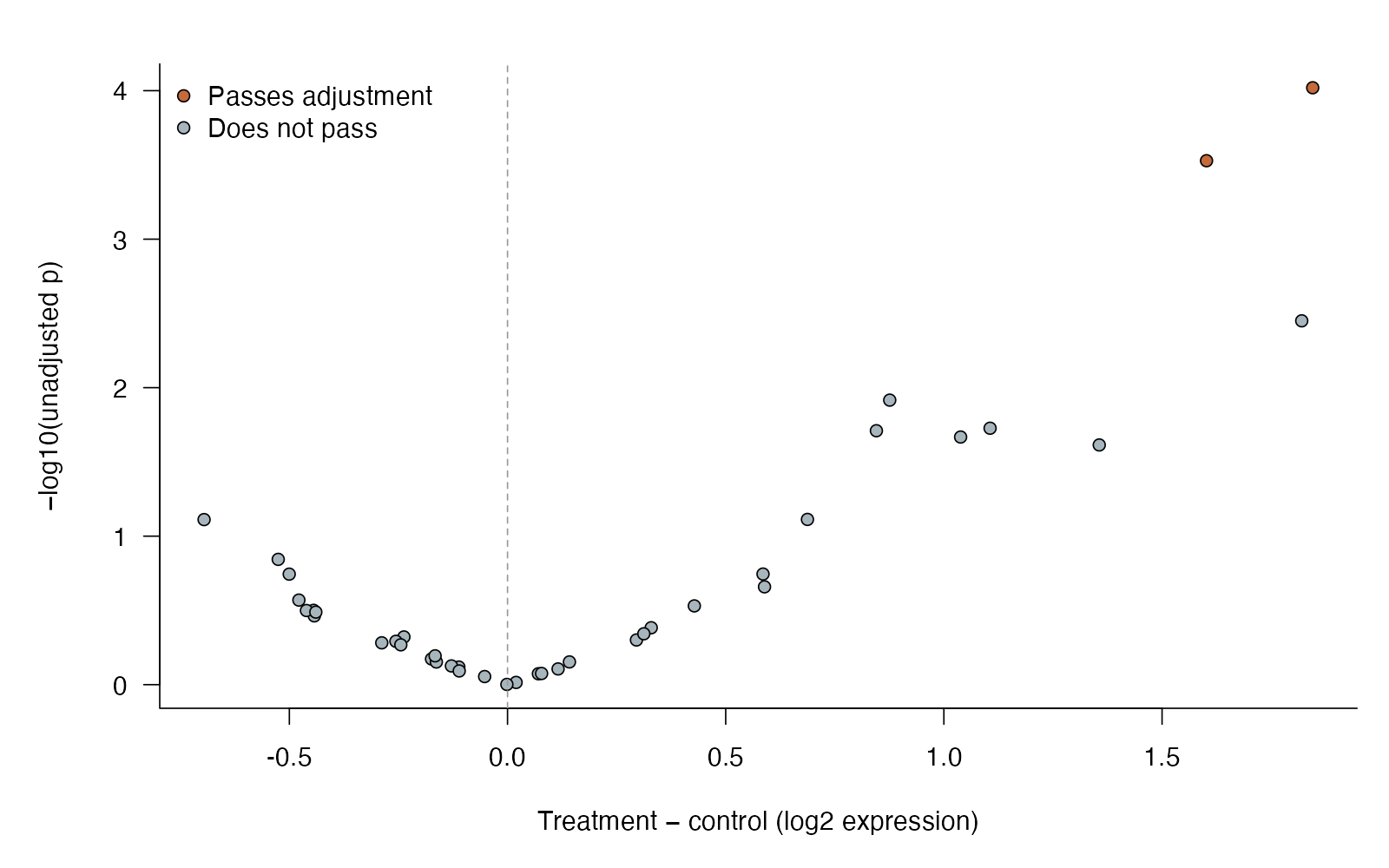
- Unadjusted p<.05: 8 genes
- Adjusted p<.05: 2 genes
- One declared family of 40 gene comparisons
Of 40 gene comparisons, 2 have Bonferroni-adjusted p-values below 0.05. With valid input tests, this rule controls the probability of at least one false positive in the family at 5%. Interpret the gene effect sizes alongside the adjusted evidence.
**Teaching point:** Bonferroni controls the chance of at least one false positive in the declared family; retain the gene effect sizes when interpreting discoveries.
### Analysis code excerpt
```r
d <- read.csv("modules/bonferroni/generated/data.csv")
p_value <- difference <- numeric(40)
for (i in 1:40) {
x <- d$expression[d$gene==i & d$treated==1]
y <- d$expression[d$gene==i & d$treated==0]
p_value[i] <- t.test(x,y)$p.value
difference[i] <- mean(x)-mean(y)
}
adjusted <- p.adjust(p_value, method="bonferroni")
result <- data.frame(gene=1:40, difference, p_value, adjusted)
```
The full script supplies package loading and any additional preparation.
### Full printed R output
```text
gene difference p_value adjusted
1 1 1.356069983 2.431656e-02 0.972662302
2 2 1.820104702 3.547859e-03 0.141914361
3 3 0.845346076 1.950008e-02 0.780003216
4 4 1.601922131 2.962924e-04 0.011851697
5 5 0.875891097 1.213253e-02 0.485301058
6 6 0.687357661 7.714434e-02 1.000000000
7 7 1.845249234 9.557971e-05 0.003823188
8 8 1.105882290 1.875913e-02 0.750365364
9 9 0.141888955 7.029532e-01 1.000000000
10 10 -0.525492608 1.433129e-01 1.000000000
11 11 -0.111584860 7.609645e-01 1.000000000
12 12 -0.500318535 1.802215e-01 1.000000000
13 13 -0.174194669 6.714101e-01 1.000000000
14 14 -0.442811468 3.442297e-01 1.000000000
15 15 -0.237449722 4.772690e-01 1.000000000
16 16 0.070743474 8.445295e-01 1.000000000
17 17 1.038355354 2.150182e-02 0.860072962
18 18 -0.478127932 2.694789e-01 1.000000000
19 19 -0.695425512 7.735015e-02 1.000000000
20 20 0.295473084 5.001759e-01 1.000000000
21 21 -0.255778461 5.105560e-01 1.000000000
22 22 -0.052458354 8.819974e-01 1.000000000
23 23 0.019658817 9.659932e-01 1.000000000
24 24 0.428118427 2.948827e-01 1.000000000
25 25 0.078072139 8.409584e-01 1.000000000
26 26 0.329322315 4.137296e-01 1.000000000
27 27 0.115868310 7.837690e-01 1.000000000
28 28 -0.128556430 7.479098e-01 1.000000000
29 29 -0.244565960 5.393038e-01 1.000000000
30 30 -0.444446000 3.158609e-01 1.000000000
31 31 -0.110704620 8.086996e-01 1.000000000
32 32 -0.163111825 7.039041e-01 1.000000000
33 33 -0.460802842 3.168194e-01 1.000000000
34 34 -0.288218696 5.228287e-01 1.000000000
35 35 0.312361668 4.543604e-01 1.000000000
36 36 -0.439299699 3.246300e-01 1.000000000
37 37 -0.001465637 9.964233e-01 1.000000000
38 38 0.588926287 2.193949e-01 1.000000000
39 39 -0.165987262 6.396148e-01 1.000000000
40 40 0.585516005 1.799847e-01 1.000000000
```
### Recreate the observations
```r
out_dir <- "modules/bonferroni/generated"
dir.create(out_dir, recursive = TRUE, showWarnings = FALSE)
set.seed(240508)
gene <- rep(1:40, each=24)
treated <- rep(rep(0:1, each=12), 40)
effect <- rep(c(rep(1.1,8), rep(0,32)), each=24)
d <- data.frame(gene, treated, expression=rnorm(960, 6+effect*treated, 1))
write.csv(d, file.path(out_dir, "data.csv"), row.names = FALSE)
```
Run the complete module from the course folder:
```sh
Rscript modules/bonferroni/analysis.R modules/bonferroni/generated
```
## Dataset 59: Benjamini–Hochberg FDR
Compare gene expression between two conditions across 40 genes.
**Family:** Multiple testing · **Rows:** 960 · **Seed:** 240509
[Saved CSV](modules/fdr/generated/data.csv) · [Full runnable R script](modules/fdr/analysis.R) · [Full-size plot](modules/fdr/generated/plot.png)
**Generating truth:** The first eight genes have true mean effects of 1.1 log2 units; the other 32 nulls are true.
**Exact generating model:** 40 genes, each with 12 control and 12 treated independent Normal observations, SD=1 log2 unit. Controls have mean 6; the first 8 genes have treatment shift 1.1; the other 32 have shift 0. Genes are independent in this simulation.
**Scientific question:** Which gene differences are supported while controlling the expected fraction of false discoveries among selected genes?
**Null being tested / estimation target:** For each gene, the treatment and control population means are equal. The adjustment changes the error criterion, not those individual nulls.
**Design and independent unit:** Each gene comparison uses 12 independent samples per condition; simulation uses independent genes.
### Columns
| Column | Meaning | Unit / type |
|---|---|---|
| gene | Gene comparison | ID |
| treated | Control=0, treated=1 | indicator |
| expression | Expression measurement | log2 units |
### Analysis from the saved dataset
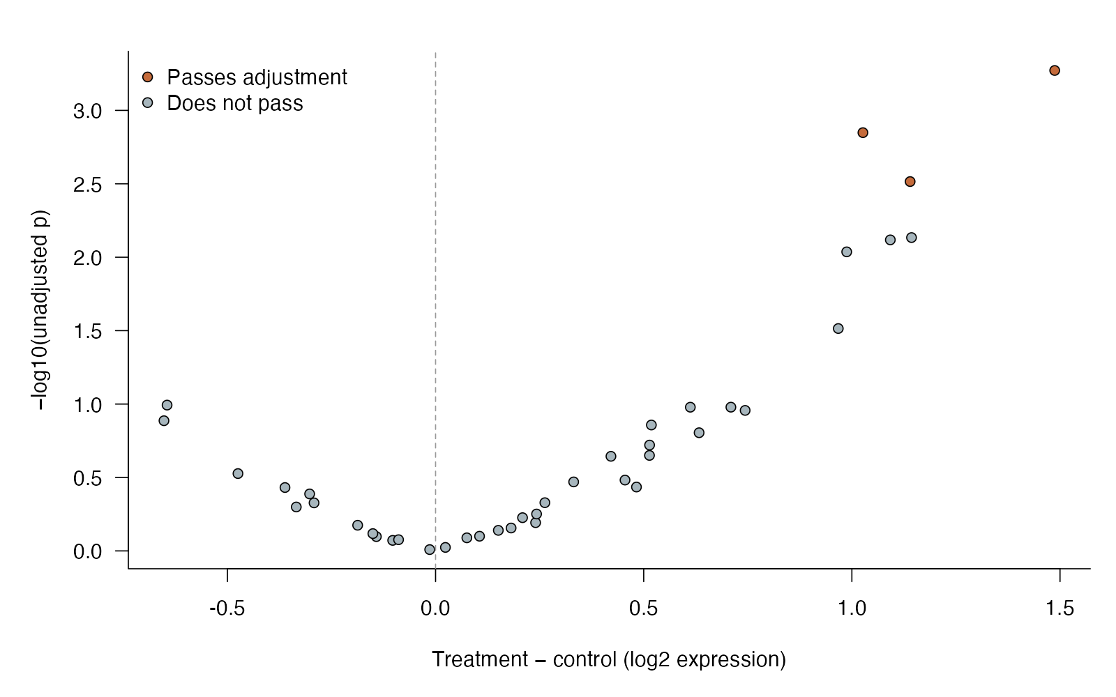
- Unadjusted p<.05: 7 genes
- Adjusted p<.05: 3 genes
- One declared family of 40 gene comparisons
Of 40 gene comparisons, 3 have BH-adjusted p-values below 0.05. Under its assumptions, this rule controls the expected false-discovery proportion among selected genes at 5%. Interpret the gene effect sizes alongside the adjusted evidence.
**Teaching point:** BH controls the expected false-discovery proportion among selected genes under its assumptions; the fraction in one particular selected set can differ.
### Analysis code excerpt
```r
d <- read.csv("modules/fdr/generated/data.csv")
p_value <- difference <- numeric(40)
for (i in 1:40) {
x <- d$expression[d$gene==i & d$treated==1]
y <- d$expression[d$gene==i & d$treated==0]
p_value[i] <- t.test(x,y)$p.value
difference[i] <- mean(x)-mean(y)
}
adjusted <- p.adjust(p_value, method="BH")
result <- data.frame(gene=1:40, difference, p_value, adjusted)
```
The full script supplies package loading and any additional preparation.
### Full printed R output
```text
gene difference p_value adjusted
1 1 0.74361874 0.1104543621 0.40165223
2 2 1.13993835 0.0030532767 0.04071036
3 3 0.63303366 0.1567432146 0.44783776
4 4 1.14326813 0.0073476739 0.06095345
5 5 0.96736406 0.0305870454 0.17478312
6 6 1.09236913 0.0076191816 0.06095345
7 7 1.48722039 0.0005346944 0.02138778
8 8 0.98760270 0.0091921923 0.06128128
9 9 0.51837432 0.1388609646 0.42726451
10 10 -0.14223887 0.7992511250 0.89242739
11 11 0.51406450 0.1902207102 0.50725523
12 12 0.70940140 0.1049898188 0.40165223
13 13 -0.30250964 0.4092528380 0.71174407
14 14 0.42126908 0.2268777905 0.53383010
15 15 0.61198019 0.1050522464 0.40165223
16 16 0.20888941 0.5939132343 0.84844748
17 17 -0.65242027 0.1298588176 0.42726451
18 18 -0.01411687 0.9796145857 0.97961459
19 19 0.24030316 0.6422998740 0.88593086
20 20 -0.64493323 0.1016113193 0.40165223
21 21 0.07513899 0.8145615887 0.89242739
22 22 -0.47464912 0.2974303246 0.66095628
23 23 0.02363298 0.9466910092 0.97096514
24 24 1.02654327 0.0014177568 0.02835514
25 25 -0.29191394 0.4709077705 0.75345243
26 26 -0.10301348 0.8478060177 0.89242739
27 27 0.18143797 0.6983414710 0.89242739
28 28 -0.18717039 0.6687974584 0.89172994
29 29 0.33171934 0.3389648607 0.67310147
30 30 0.15073943 0.7246670673 0.89242739
31 31 0.51380224 0.2236912675 0.53383010
32 32 -0.08888316 0.8389536027 0.89242739
33 33 0.26256464 0.4695329863 0.75345243
34 34 -0.15063432 0.7623551098 0.89242739
35 35 -0.36171374 0.3702058103 0.67310147
36 36 0.45507254 0.3293200199 0.67310147
37 37 -0.33460383 0.5022342610 0.77266809
38 38 0.24260469 0.5607670894 0.83076606
39 39 0.48258110 0.3672953546 0.67310147
40 40 0.10560952 0.7943725893 0.89242739
```
### Recreate the observations
```r
out_dir <- "modules/fdr/generated"
dir.create(out_dir, recursive = TRUE, showWarnings = FALSE)
set.seed(240509)
gene <- rep(1:40, each=24)
treated <- rep(rep(0:1, each=12), 40)
effect <- rep(c(rep(1.1,8), rep(0,32)), each=24)
d <- data.frame(gene, treated, expression=rnorm(960, 6+effect*treated, 1))
write.csv(d, file.path(out_dir, "data.csv"), row.names = FALSE)
```
Run the complete module from the course folder:
```sh
Rscript modules/fdr/analysis.R modules/fdr/generated
```
## Dataset 60: Principal component analysis
Four correlated morphological traits are measured in beetles from three ecotypes.
**Family:** Multivariate exploration · **Rows:** 75 · **Seed:** 240510
[Saved CSV](modules/pca/generated/data.csv) · [Full runnable R script](modules/pca/analysis.R) · [Full-size plot](modules/pca/generated/plot.png)
**Generating truth:** Groups differ in body-size means and antenna shifts; all traits share a common body-size component.
**Exact generating model:** 75 beetles: 25 per ecotype. Body size is Normal(mean 12,14,13 mm by Forest,Grassland,Dune; SD 1.2). Wing=1.3×size+Normal(0,1); femur=0.45×size+Normal(0,0.4); antenna=0.7×size+ecotype shift(0,1,−1)+Normal(0,0.5). All errors independent.
**Scientific question:** Which combinations of traits summarize the most variation?
**Null being tested / estimation target:** The target is a set of linear trait combinations that explain the most variance; PCA itself does not test a null hypothesis.
**Design and independent unit:** 25 independent beetles per ecotype; four traits on each individual.
### Columns
| Column | Meaning | Unit / type |
|---|---|---|
| ecotype | Known source habitat | category |
| body_mm | body | mm |
| wing_mm | wing | mm |
| femur_mm | femur | mm |
| antenna_mm | antenna | mm |
### Analysis from the saved dataset
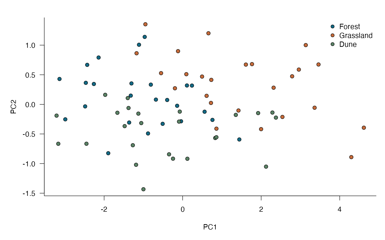
- PC1 accounts for 84.3% of variance
- PC2 accounts for 8.6%
- Variables centered and scaled
The first two principal components account for 92.9% of the standardized trait variance. Separation is descriptive; PCA does not test a population difference.
**Teaching point:** PCA uses the measurements, not class labels, to construct the axes.
### Analysis code excerpt
```r
d <- read.csv("modules/pca/generated/data.csv")
z <- d[c("body_mm","wing_mm","femur_mm","antenna_mm")]
result <- prcomp(z, center=TRUE, scale.=TRUE)
variance <- result$sdev^2/sum(result$sdev^2)
```
The full script supplies package loading and any additional preparation.
### Full printed R output
```text
Standard deviations (1, .., p=4):
[1] 1.8360217 0.5857306 0.4563007 0.2788073
Rotation (n x k) = (4 x 4):
PC1 PC2 PC3 PC4
body_mm 0.5283830 -0.09689995 0.05098935 -0.8419156
wing_mm 0.4805746 -0.77094271 -0.17456589 0.3797659
femur_mm 0.5007526 0.30369527 0.74286006 0.3243069
antenna_mm 0.4889849 0.55138637 -0.64427150 0.2044041
```
### Recreate the observations
```r
out_dir <- "modules/pca/generated"
dir.create(out_dir, recursive = TRUE, showWarnings = FALSE)
set.seed(240510)
ecotype <- rep(c("Forest", "Grassland", "Dune"), each=25)
size <- rnorm(75, rep(c(12,14,13),each=25), 1.2)
d <- data.frame(ecotype, body_mm=size,
wing_mm=1.3*size+rnorm(75,0,1), femur_mm=.45*size+rnorm(75,0,.4),
antenna_mm=.7*size+rep(c(0,1,-1),each=25)+rnorm(75,0,.5))
write.csv(d, file.path(out_dir, "data.csv"), row.names = FALSE)
```
Run the complete module from the course folder:
```sh
Rscript modules/pca/analysis.R modules/pca/generated
```
## Dataset 61: Classical multidimensional scaling
Four correlated morphological traits are measured in beetles from three ecotypes.
**Family:** Multivariate exploration · **Rows:** 75 · **Seed:** 240511
[Saved CSV](modules/mds/generated/data.csv) · [Full runnable R script](modules/mds/analysis.R) · [Full-size plot](modules/mds/generated/plot.png)
**Generating truth:** Groups differ in body-size means and antenna shifts; all traits share a common body-size component.
**Exact generating model:** 75 beetles: 25 per ecotype. Body size is Normal(mean 12,14,13 mm by Forest,Grassland,Dune; SD 1.2). Wing=1.3×size+Normal(0,1); femur=0.45×size+Normal(0,0.4); antenna=0.7×size+ecotype shift(0,1,−1)+Normal(0,0.5). All errors independent.
**Scientific question:** Can a low-dimensional map preserve the chosen between-individual distances?
**Null being tested / estimation target:** The target is a low-dimensional configuration that preserves the chosen distances; this map is not itself a hypothesis test.
**Design and independent unit:** 25 independent beetles per ecotype; four traits on each individual.
### Columns
| Column | Meaning | Unit / type |
|---|---|---|
| ecotype | Known source habitat | category |
| body_mm | body | mm |
| wing_mm | wing | mm |
| femur_mm | femur | mm |
| antenna_mm | antenna | mm |
### Analysis from the saved dataset
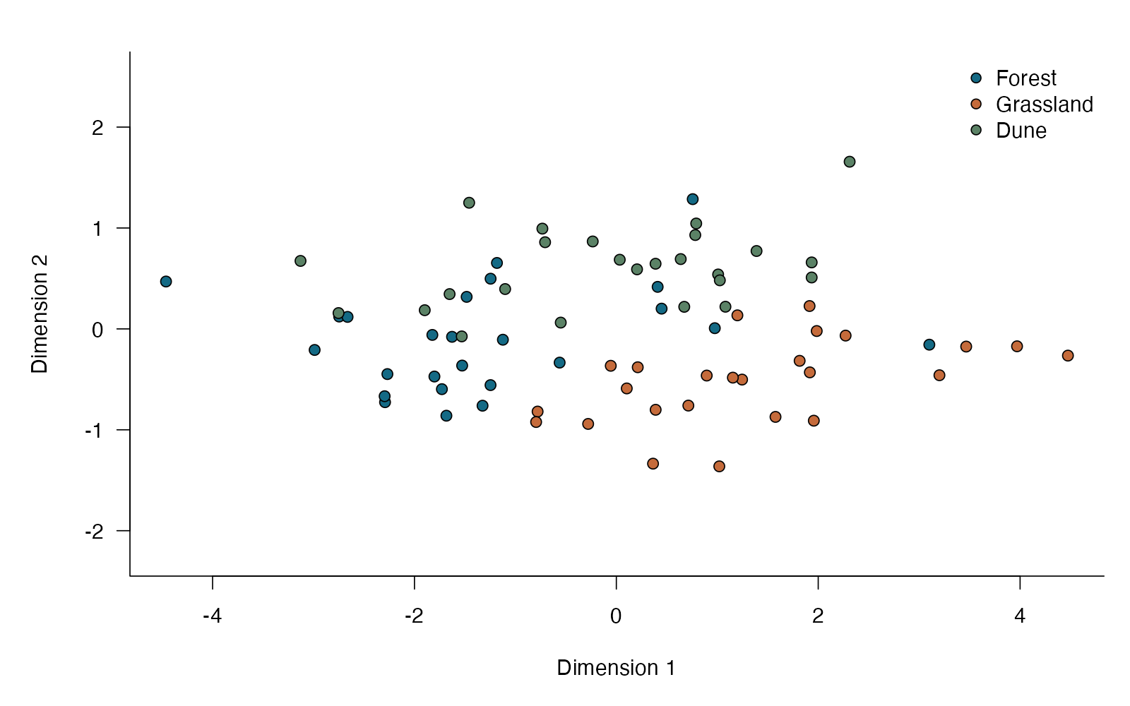
- Two-dimensional goodness of fit: 0.920
- Euclidean distances between standardized traits
- Closer points have more similar trait combinations
The two-dimensional configuration has a goodness-of-fit measure of 0.920 for the supplied distances. Its axes summarize distances; their signs and orientation have no fixed biological meaning.
**Teaching point:** Distance choice defines what counts as similar.
### Analysis code excerpt
```r
d <- read.csv("modules/mds/generated/data.csv")
z <- scale(d[c("body_mm","wing_mm","femur_mm","antenna_mm")])
distance <- dist(z)
result <- cmdscale(distance, k=2, eig=TRUE)
```
The full script supplies package loading and any additional preparation.
### Full printed R output
```text
$points
[,1] [,2]
[1,] 0.97540338 0.007130556
[2,] -4.46130829 0.469609156
[3,] -1.24571197 0.497452164
[4,] -1.72828046 -0.597133304
[5,] -2.74594570 0.122395278
[6,] -2.26815563 -0.447789896
[7,] -1.12397958 -0.107186606
[8,] -2.29155329 -0.726311080
[9,] -1.80227000 -0.471975030
[10,] -0.56171783 -0.334092884
[11,] -1.18275802 0.653631090
[12,] -1.48299577 0.317510437
[13,] -1.62765057 -0.078355363
[14,] -2.98896933 -0.208697033
[15,] -1.52757541 -0.363367937
[16,] -1.24637429 -0.557080003
[17,] -1.68366709 -0.860288254
[18,] 0.75666938 1.285941982
[19,] -2.29549992 -0.667152081
[20,] -2.66289688 0.118922324
[21,] 3.10082130 -0.156332459
[22,] -1.82282364 -0.059656139
[23,] 0.40921175 0.416657106
[24,] -1.32552072 -0.761149165
[25,] 0.44845870 0.200823791
[26,] 0.10324130 -0.589977555
[27,] 1.19923123 0.134419369
[28,] 3.96984785 -0.172448876
[29,] 2.27126118 -0.066311361
[30,] 1.91711754 -0.430709984
[31,] 0.89544237 -0.462383205
[32,] -0.78009775 -0.819192745
[33,] 1.95641125 -0.909672844
[34,] -0.79468191 -0.922655152
[35,] -0.05522046 -0.365612822
[36,] 1.91428844 0.226624485
[37,] 3.20090994 -0.459201925
[38,] 0.21205988 -0.380048608
[39,] 1.02003356 -1.362147284
[40,] 1.24568281 -0.502301932
[41,] 1.57679589 -0.872085050
[42,] 1.81592643 -0.316351601
[43,] -0.27934197 -0.941706918
[44,] 0.71348105 -0.759967619
[45,] 0.38942396 -0.801572292
[46,] 4.47393929 -0.264713577
[47,] 1.98517161 -0.021157208
[48,] 0.36349297 -1.335409653
[49,] 1.15444022 -0.482976416
[50,] 3.46599888 -0.175119031
[51,] -1.53157106 -0.074276676
[52,] 0.78199752 0.930207230
[53,] 1.93515071 0.509660813
[54,] -0.70579706 0.859092352
[55,] 1.93518403 0.658875892
[56,] 0.67278208 0.218760206
[57,] 2.31127845 1.656886824
[58,] 1.38891081 0.771957279
[59,] -3.12887039 0.673693604
[60,] 0.20500793 0.590338474
[61,] 1.08079324 0.219675988
[62,] -1.65195396 0.345045343
[63,] -0.23402694 0.866576022
[64,] 0.63783338 0.691868939
[65,] 0.03377474 0.685551771
[66,] -0.73276347 0.993763279
[67,] 0.38852270 0.645752563
[68,] 1.00849774 0.539426058
[69,] -1.10164072 0.394921013
[70,] -2.75230520 0.157078109
[71,] -1.89821525 0.185367845
[72,] 1.02526505 0.481524596
[73,] -0.55076836 0.062510038
[74,] 0.79132930 1.044617787
[75,] -1.45818095 1.250297811
$eig
[1] 2.415403e+02 3.065253e+01 1.922729e+01 4.579862e+00 9.815933e-15
[6] 7.269084e-15 6.521041e-15 6.457920e-15 5.351543e-15 5.024629e-15
[11] 3.536685e-15 3.224538e-15 3.067886e-15 2.784960e-15 2.781320e-15
[16] 2.715877e-15 2.455016e-15 2.311272e-15 2.161329e-15 1.958721e-15
[21] 1.911807e-15 1.878351e-15 1.848735e-15 1.841280e-15 1.815672e-15
[26] 1.404475e-15 1.240902e-15 1.143682e-15 8.747429e-16 6.569501e-16
[31] 5.432930e-16 5.345057e-16 3.332429e-16 2.448202e-16 2.198298e-16
[36] 1.350057e-16 1.320982e-16 7.297038e-17 6.174247e-18 -1.292171e-16
[41] -2.390654e-16 -3.186937e-16 -3.438659e-16 -3.717135e-16 -4.448662e-16
[46] -4.953244e-16 -5.242173e-16 -5.484482e-16 -5.981108e-16 -6.448906e-16
[51] -6.998647e-16 -7.125050e-16 -7.285133e-16 -8.590374e-16 -9.645182e-16
[56] -9.755598e-16 -1.171510e-15 -1.301264e-15 -1.519557e-15 -1.560846e-15
[61] -2.906036e-15 -3.566509e-15 -3.793373e-15 -4.033947e-15 -4.147306e-15
[66] -4.299794e-15 -6.382293e-15 -6.885932e-15 -6.931247e-15 -7.223042e-15
[71] -7.241831e-15 -1.007704e-14 -1.271357e-14 -1.335275e-14 -5.515095e-14
$x
NULL
$ac
[1] 0
$GOF
[1] 0.9195704 0.9195704
```
### Recreate the observations
```r
out_dir <- "modules/mds/generated"
dir.create(out_dir, recursive = TRUE, showWarnings = FALSE)
set.seed(240511)
ecotype <- rep(c("Forest", "Grassland", "Dune"), each=25)
size <- rnorm(75, rep(c(12,14,13),each=25), 1.2)
d <- data.frame(ecotype, body_mm=size,
wing_mm=1.3*size+rnorm(75,0,1), femur_mm=.45*size+rnorm(75,0,.4),
antenna_mm=.7*size+rep(c(0,1,-1),each=25)+rnorm(75,0,.5))
write.csv(d, file.path(out_dir, "data.csv"), row.names = FALSE)
```
Run the complete module from the course folder:
```sh
Rscript modules/mds/analysis.R modules/mds/generated
```
## Dataset 62: Linear discriminant analysis
Four correlated morphological traits are measured in beetles from three ecotypes.
**Family:** Multivariate exploration · **Rows:** 75 · **Seed:** 240512
[Saved CSV](modules/lda/generated/data.csv) · [Full runnable R script](modules/lda/analysis.R) · [Full-size plot](modules/lda/generated/plot.png)
**Generating truth:** Groups differ in body-size means and antenna shifts; all traits share a common body-size component.
**Exact generating model:** 75 beetles: 25 per ecotype. Body size is Normal(mean 12,14,13 mm by Forest,Grassland,Dune; SD 1.2). Wing=1.3×size+Normal(0,1); femur=0.45×size+Normal(0,0.4); antenna=0.7×size+ecotype shift(0,1,−1)+Normal(0,0.5). All errors independent.
**Scientific question:** How well can measured traits predict known group membership?
**Null being tested / estimation target:** The target is predictive classification of known ecotypes; this example estimates validation accuracy rather than testing a null hypothesis.
**Design and independent unit:** 25 independent beetles per ecotype; four traits on each individual.
### Columns
| Column | Meaning | Unit / type |
|---|---|---|
| ecotype | Known source habitat | category |
| body_mm | body | mm |
| wing_mm | wing | mm |
| femur_mm | femur | mm |
| antenna_mm | antenna | mm |
### Analysis from the saved dataset
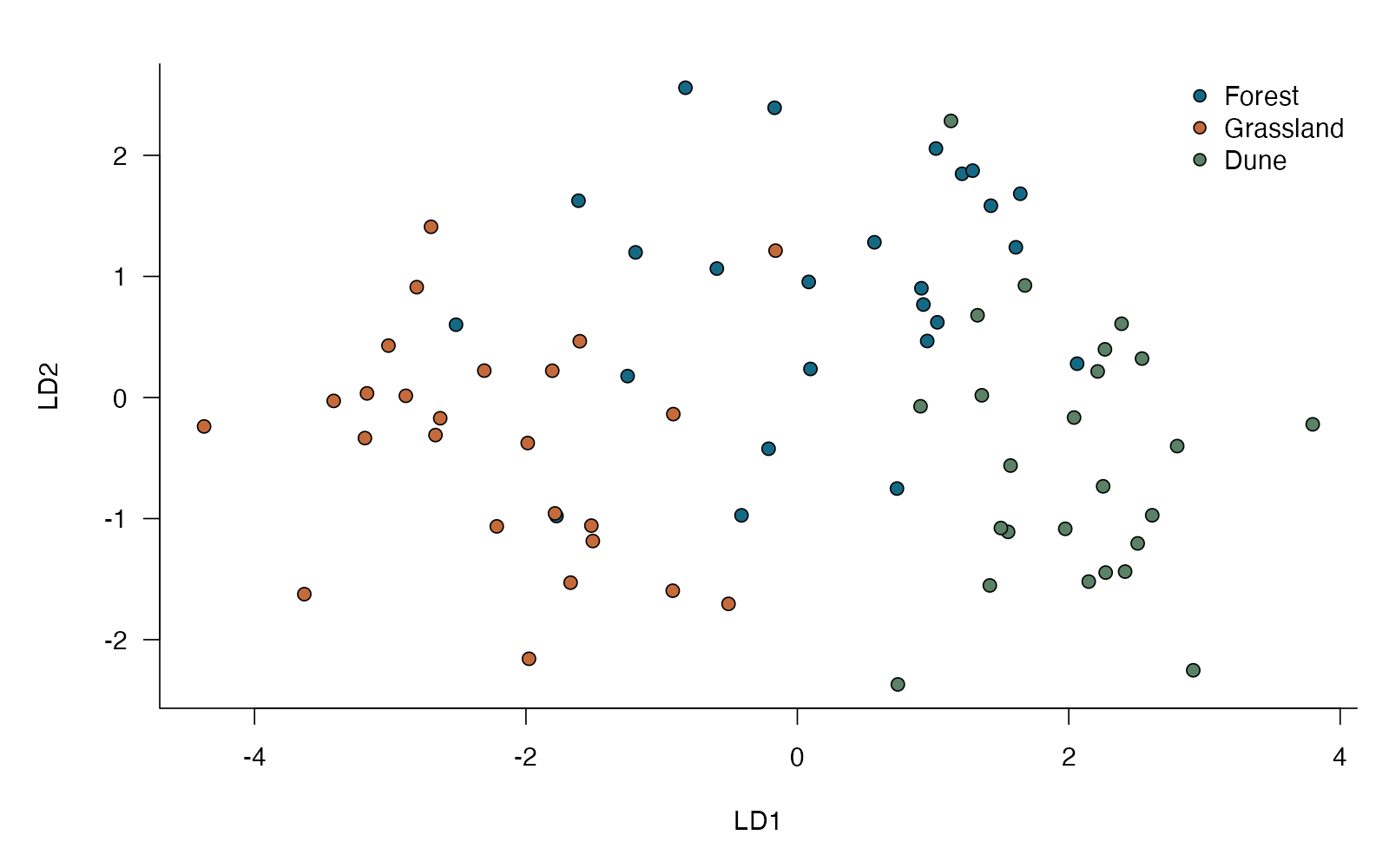
- Leave-one-out classification accuracy: 82.7%
- Three known ecotype labels used during training
- Equal group sizes in this example
Leave-one-out classification accuracy is 82.7% for these three ecotypes. This is a prediction exercise using known class labels, not an unsupervised discovery or a significance test.
**Teaching point:** LDA uses the labels to find discrimination; separation on training data is not validation.
### Analysis code excerpt
```r
d <- read.csv("modules/lda/generated/data.csv")
result <- MASS::lda(ecotype ~ body_mm + wing_mm + femur_mm + antenna_mm, data=d)
cv <- MASS::lda(ecotype ~ body_mm + wing_mm + femur_mm + antenna_mm, data=d, CV=TRUE)
accuracy <- mean(cv$class==d$ecotype)
```
The full script supplies package loading and any additional preparation.
### Full printed R output
```text
Call:
lda(ecotype ~ body_mm + wing_mm + femur_mm + antenna_mm, data = d)
Prior probabilities of groups:
Dune Forest Grassland
0.3333333 0.3333333 0.3333333
Group means:
body_mm wing_mm femur_mm antenna_mm
Dune 12.70929 17.02713 5.706581 7.915556
Forest 11.99869 15.71095 5.328634 8.397726
Grassland 13.90283 17.92353 6.288135 10.870551
Coefficients of linear discriminants:
LD1 LD2
body_mm 1.01499407 -0.78013116
wing_mm 0.10976514 -0.43360845
femur_mm 0.09092525 -0.08365976
antenna_mm -1.89182813 0.50613401
Proportion of trace:
LD1 LD2
0.8823 0.1177
```
### Recreate the observations
```r
out_dir <- "modules/lda/generated"
dir.create(out_dir, recursive = TRUE, showWarnings = FALSE)
set.seed(240512)
ecotype <- rep(c("Forest", "Grassland", "Dune"), each=25)
size <- rnorm(75, rep(c(12,14,13),each=25), 1.2)
d <- data.frame(ecotype, body_mm=size,
wing_mm=1.3*size+rnorm(75,0,1), femur_mm=.45*size+rnorm(75,0,.4),
antenna_mm=.7*size+rep(c(0,1,-1),each=25)+rnorm(75,0,.5))
write.csv(d, file.path(out_dir, "data.csv"), row.names = FALSE)
```
Run the complete module from the course folder:
```sh
Rscript modules/lda/analysis.R modules/lda/generated
```
## Dataset 63: Count and rate GEE
Microbial ecologists count bacterial colonies in repeated water samples from experimental pond mesocosms.
**Family:** Dependent observations · **Rows:** 360 · **Seed:** 1401
[Saved CSV](modules/count_gee/generated/data.csv) · [Full runnable R script](modules/count_gee/analysis.R) · [Full-size plot](modules/count_gee/generated/plot.png)
**Generating truth:** The exact population-average Warm / Ambient rate ratio is exp(0.45), approximately 1.568; the equal-rate null is false. Each week multiplies the marginal rate by exp(0.1), approximately 1.105. Marginal count variance is mu + 0.5 × mu squared. The working exchangeable correlation is approximate, while the specified marginal mean is exact.
**Exact generating model:** Ninety independent mesocosms (45 Ambient, 45 Warm) are sampled at weeks 0, 1, 2, and 3. Each volume is Uniform(0.5, 1.5) mL. The marginal expected count is mu = volume × exp(2.2 + 0.45 × Warm + 0.1 × week). Each mesocosm has one independent Gamma(shape 2, rate 2) multiplier, with mean 1 and variance 0.5. Conditional counts are independent Poisson(mu × multiplier), so repeated observations share the multiplier. No rounding or censoring is added.
**Scientific question:** Does warming change the population-average colony rate after accounting for week and sampled volume?
**Null being tested / estimation target:** The warming coefficient is zero: population-average colony rates are equal at the same week and exposure.
**Design and independent unit:** Ninety independent mesocosms, 45 per temperature treatment, are sampled at weeks 0–3. Each sample has a known plated volume.
### Columns
| Column | Meaning | Unit / type |
|---|---|---|
| mesocosm | Independent experimental mesocosm and repeated-sample cluster | ID |
| week | Sampling time since experiment began | week |
| treatment | Assigned ambient or warmed temperature | category |
| volume_ml | Sampled/plated water volume: the count exposure | mL |
| colonies | Observed colony count in the plated sample | count |
### Analysis from the saved dataset
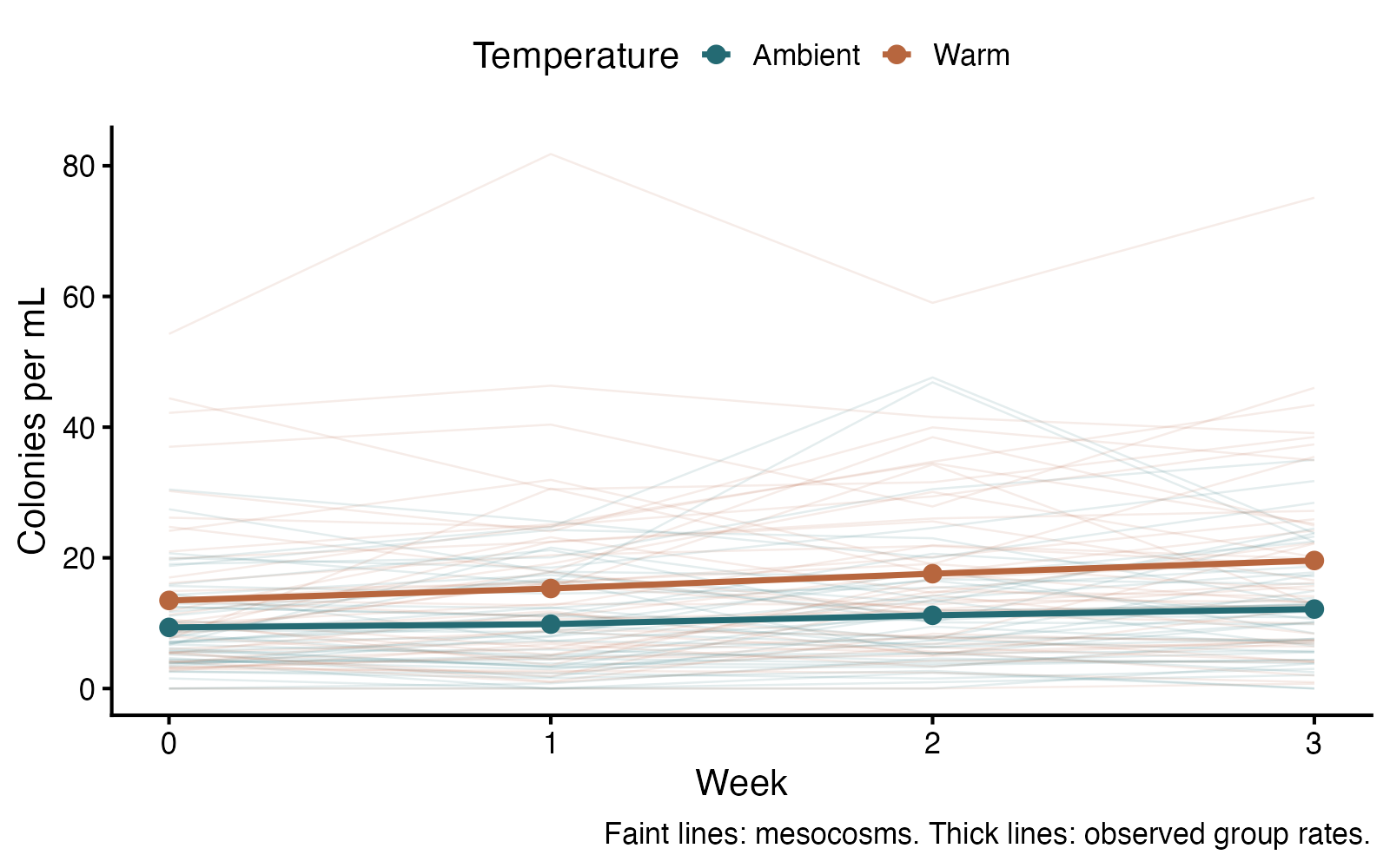
- Independent mesocosms: 90; observations: 360
- Population-average Warm / Ambient rate ratio = 1.580
- 95% robust CI: 1.175 to 2.123
- Robust Wald p = 0.00243
- Working correlation estimate = 0.816
The population-average colony rate in warmed mesocosms was 1.58 times the ambient rate (95% robust CI 1.18 to 2.12; Wald p = 0.00243), adjusting for week and sampled volume. The 90 mesocosms are the independent units; the model accounts for their repeated samples.
**Teaching point:** GEE estimates a population-average rate ratio and uses mesocosms as independent units. The offset accounts for exposure; robust uncertainty accommodates the extra variation and repeated observations.
### Analysis code excerpt
```r
d <- read.csv("modules/count_gee/generated/data.csv")
d$treatment <- factor(d$treatment, levels = c("Ambient", "Warm"))
d <- d[order(d$mesocosm, d$week), ]
fit <- geepack::geeglm(colonies ~ treatment + week + offset(log(volume_ml)),
id = mesocosm, data = d, family = poisson(link = "log"),
corstr = "exchangeable", std.err = "san.se")
b <- coef(fit)["treatmentWarm"]
se <- sqrt(vcov(fit)["treatmentWarm", "treatmentWarm"])
rate_ratio <- exp(b)
ci <- exp(b + c(-1, 1) * 1.96 * se)
p_value <- 2 * pnorm(abs(b / se), lower.tail = FALSE)
```
The full script supplies package loading and any additional preparation.
### Full printed R output
```text
Call:
geepack::geeglm(formula = colonies ~ treatment + week + offset(log(volume_ml)),
family = poisson(link = "log"), data = d, id = mesocosm,
corstr = "exchangeable", std.err = "san.se")
Coefficients:
Estimate Std.err Wald Pr(>|W|)
(Intercept) 2.20660 0.10491 442.355 < 2e-16 ***
treatmentWarm 0.45715 0.15078 9.193 0.00243 **
week 0.10817 0.01322 66.937 3.33e-16 ***
---
Signif. codes: 0 ‘***’ 0.001 ‘**’ 0.01 ‘*’ 0.05 ‘.’ 0.1 ‘ ’ 1
Correlation structure = exchangeable
Estimated Scale Parameters:
Estimate Std.err
(Intercept) 7.602 1.51
Link = identity
Estimated Correlation Parameters:
Estimate Std.err
alpha 0.8161 0.04783
Number of clusters: 90 Maximum cluster size: 4
```
### Recreate the observations
```r
output_dir <- "modules/count_gee/generated"
dir.create(output_dir, recursive = TRUE, showWarnings = FALSE)
set.seed(1401)
mesocosm <- rep(1:90, each = 4)
week <- rep(0:3, 90)
treatment <- rep(rep(c("Ambient", "Warm"), each = 45), each = 4)
volume_ml <- runif(360, .5, 1.5)
shared_rate <- rgamma(90, shape = 2, rate = 2)
mu <- volume_ml * exp(2.2 + .45 * (treatment == "Warm") + .1 * week)
colonies <- rpois(360, mu * shared_rate[mesocosm])
d <- data.frame(mesocosm, week, treatment, volume_ml, colonies)
write.csv(d, file.path(output_dir, "data.csv"), row.names = FALSE)
```
Run the complete module from the course folder:
```sh
Rscript modules/count_gee/analysis.R modules/count_gee/generated
```
## Reproducibility notes
Each module owns its fixed seed, simulation, saved CSV, plot, and actual analysis output. Identifiers are local to the module. Generating-model descriptions state rounding, dependence, censoring, or deliberate unusual observations.
The guide reads saved data and result files without rerunning simulations or analyses. Run the course builder or changed module scripts before refreshing the guide. The catalog includes file checksums for this build.
```r
source("build_instructor_guide.R")
build_instructor_guide(".")
```
Built 2026-09-23 22:54 CDT from 63 saved module datasets. All discovered modules are included.